Transcription
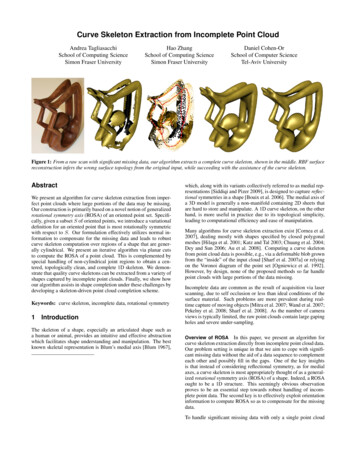
Curve Skeleton Extraction from Incomplete Point CloudAndrea TagliasacchiSchool of Computing ScienceSimon Fraser UniversityHao ZhangSchool of Computing ScienceSimon Fraser UniversityDaniel Cohen-OrSchool of Computer ScienceTel-Aviv UniversityFigure 1: From a raw scan with significant missing data, our algorithm extracts a complete curve skeleton, shown in the middle. RBF surfacereconstruction infers the wrong surface topology from the original input, while succeeding with the assistance of the curve skeleton.AbstractWe present an algorithm for curve skeleton extraction from imperfect point clouds where large portions of the data may be missing.Our construction is primarily based on a novel notion of generalizedrotational symmetry axis (ROSA) of an oriented point set. Specifically, given a subset S of oriented points, we introduce a variationaldefinition for an oriented point that is most rotationally symmetricwith respect to S. Our formulation effectively utilizes normal information to compensate for the missing data and leads to robustcurve skeleton computation over regions of a shape that are generally cylindrical. We present an iterative algorithm via planar cutsto compute the ROSA of a point cloud. This is complemented byspecial handling of non-cylindrical joint regions to obtain a centered, topologically clean, and complete 1D skeleton. We demonstrate that quality curve skeletons can be extracted from a variety ofshapes captured by incomplete point clouds. Finally, we show howour algorithm assists in shape completion under these challenges bydeveloping a skeleton-driven point cloud completion scheme.Keywords: curve skeleton, incomplete data, rotational symmetry1IntroductionThe skeleton of a shape, especially an articulated shape such asa human or animal, provides an intuitive and effective abstractionwhich facilitates shape understanding and manipulation. The bestknown skeletal representation is Blum’s medial axis [Blum 1967],which, along with its variants collectively referred to as medial representations [Siddiqi and Pizer 2009], is designed to capture reflectional symmetries in a shape [Bouix et al. 2006]. The medial axis ofa 3D model is generally a non-manifold containing 2D sheets thatare hard to store and manipulate. A 1D curve skeleton, on the otherhand, is more useful in practice due to its topological simplicity,leading to computational efficiency and ease of manipulation.Many algorithms for curve skeleton extraction exist [Cornea et al.2007], dealing mostly with shapes specified by closed polygonalmeshes [Hilaga et al. 2001; Katz and Tal 2003; Chuang et al. 2004;Dey and Sun 2006; Au et al. 2008]. Computing a curve skeletonfrom point cloud data is possible, e.g., via a deformable blob grownfrom the “inside” of the input cloud [Sharf et al. 2007a] or relyingon the Voronoi diagram of the point set [Ogniewicz et al. 1992].However, by design, none of the proposed methods so far handlepoint clouds with large portions of the data missing.Incomplete data are common as the result of acquisition via laserscanning, due to self occlusion or less than ideal conditions of thesurface material. Such problems are more prevalent during realtime capture of moving objects [Mitra et al. 2007; Wand et al. 2007;Pekelny et al. 2008; Sharf et al. 2008]. As the number of cameraviews is typically limited, the raw point clouds contain large gapingholes and severe under-sampling.In this paper, we present an algorithm forcurve skeleton extraction directly from incomplete point cloud data.Our problem setting is unique in that we aim to cope with significant missing data without the aid of a data sequence to complementeach other and possibly fill in the gaps. One of the key insightsis that instead of considering reflectional symmetry, as for medialaxes, a curve skeleton is most appropriately thought of as a generalized rotational symmetry axis (ROSA) of a shape. Indeed, a ROSAought to be a 1D structure. This seemingly obvious observationproves to be an essential step towards robust handling of incomplete point data. The second key is to effectively exploit orientationinformation to compute ROSA so as to compensate for the missingdata.Overview of ROSATo handle significant missing data with only a single point cloud
Figure 2: ROSA definition for a set of oriented points in 3D. Left:Optimal direction (red arrow) minimizes sum of angular variationswith the surrounding normals. Right: Optimal point (red dot) minimizes sum of projected distances to the normal extensions.Figure 3: Stability of ROSA point position and orientation withmore than half of the points missing.available, an appropriate shape prior is necessary. A generalpremise of our approach is that the shapes of interest should be covered by generally cylindrical regions except at their joints. This is areasonable assumption as only such shapes would admit meaningful curve skeletons; a serving plate, baseball cap, or bowling ball,for example, do not belong to this category and they possess nonatural curve skeletons. ROSA is designed to skeletonize generallycylindrical regions, even with significant missing data.To compute ROSA, we take advantage of available point normalsand introduce a variational formulation which works on a local subset S of oriented samples in the input point cloud. We define anoriented point p (xp , vp ), called a ROSA point, with position xpand normal vp , that is most rotationally symmetric about S. Ourdefinition applies to 3D quantities and it requires that1. the orientation vp minimizes the variance of the angles between vp and the normals in S. In other words, vp is to makethe same angle with these normals as much as possible, consistent with the notion of rotational symmetry;2. the position xp minimizes the sum of squared distances to theline extensions of the point normals in S.Figure 2 illustrates our definition and Figure 3 shows it at workwith significant missing data. One can immediately recognize thedifference between our formulations and the use of average normalor centroid — both are sensitive to missing data.Figure 4 reinforces the point that orientation information can effectively compensate for missing data in curve skeleton extraction. Relying on point orientation for shape inference has been a commonpractice in several other contexts, such as neighborhood identification via Mahalanobis distance [Amenta and Kil 2004; Lehtinenet al. 2008] and surface reconstruction with the assistance of pointnormals [Carr et al. 2001; Kazhdan et al. 2006].Building on the local ROSA formulation, we present an iterativeprocedure via planar cuts to locate the best subset S for derivingthe rotational symmetry axis of the whole point cloud. It is interesting to note that if such procedures were to be applied to a 2Dshape, we would arrive at a point on the symmetry set of the shapeboundary [Giblin and Brassett 1985], of which the medial axis is asubset. This connection is discussed further in Section 3.Figure 4: Orientation information compensates for missing data.Left: With missing samples from two touch circles and no normals,the computed centroid (green dot) leads to a wrong interpretationof the data. Right: Sample normals reveal two clusters, leading totwo ROSA points (red dots). The correct shape can be inferred.Contributions The main contributions of our work include anovel definition of generalized rotational symmetry axis for a pointset that is: (i) designed to model generally cylindrical regions of ashape, and (ii) robust to missing data. We develop a curve skeleton extraction algorithm from incomplete point clouds based onrecursive planar cuts and local ROSA construction, as well as ascheme to robustly detect and skeletonize the non-cylindrical jointregions of a shape. The computed curve skeleton is complete, despite a potentially incomplete data source, and it is guaranteed to bea 1D structure with associated correspondence to points in the inputcloud. We demonstrate experimentally that quality curve skeletonscan be constructed from a variety of shapes under imperfect dataconditions. Finally, we show an application of our algorithm forshape completion under significant missing data; see Figure 1.2Related workSkeletons are effective shape abstractions that have been used invarious applications including mesh segmentation [Li et al. 2001;Au et al. 2008], animation [Lewis et al. 2000], and shape matching [Hilaga et al. 2001]. We focus on 1D curve skeletons embeddedin 3D. For a coverage on medial axis and other higher dimensionalmedial representations, we point out the recent book by Siddiqi andPizer [2009]. There are many existing algorithms for curve skeleton extraction and we only mention a subset. For the rest, we referthe reader to the recent survey by Cornea and Min [2007].The field-based approach to curve skeleton extraction relies on anEuclidean distance field [Malandain and Fernández-Vidal 1998] oran implicit potential field [Chuang et al. 2004] corresponding to theinput shape, resulting in a voxelized representation of the internalvolume. The skeleton is then computed via volumetric thinning,ridge extraction, or force following along the ridges of a potentialfield. These methods generally require clear knowledge about theinterior of the input shape, making them inapplicable to incompletedata. The recent work of Au et al. [2008] shares some flavors withfield-based methods; it skeletonizes a shape by shrinking it usingconstrained Laplacian smoothing. Excellent results are obtained,but they can only come from watertight meshes, since Laplaciansmoothing requires mesh connectivity and a full model is needed tobalance the shrinking process so as to obtain a centered skeleton.Other works which require complete meshes as input include Liet al. [2001] which uses mesh decimation, the segmentation-basedapproach, e.g., Katz and Tal [2003], and topology-driven methods,e.g., via Reeb graphs [Hilaga et al. 2001; Patane et al. 2008], whichextract and link critical points of a function over the mesh surface.The latter rely on geodesic distances, which are difficult to obtainon a point cloud with significant missing data. Geodesic distancesalso play a key role in the work of Dey and Sun [2006] where theydefine a medial geodesic function over the medial axis of a shape toskeletonize the medial axis into a 1D structure.
(a)(b)(c)(d)(e)(f)Figure 5: Overview of our algorithm. (a) Input point cloud with a joint (blue). (b) Optimal cutting plane and relevant neighborhood points(blue) anchored at a point cloud sample (red particle). (c) Skeletal cloud after ROSA and joint recovery. (d) After thinning with branch(green) and joint (blue) identification. (e) After re-centering, still a skeletal cloud. (f) The final 1D curve skeleton.Recently, skeleton extraction from a sequence of deformingmeshes [James and Twigg 2005; de Aguiar et al. 2008] has beenof interest. These methods utilize vertex correspondence acrossframes and assumptions on motion, e.g., piecewise rigidity, to extract the skeleton or bones from complete data. In our problem setting, the input is a single point cloud with significant missing data.Shape completion prior to skeletonization, e.g., via RBF [Carr et al.2001], can be a means to handle incomplete point clouds. However,these surface reconstruction schemes are not designed to cope withsignificant missing data. In such cases, user intervention is oftennecessary to clarify object topology [Sharf et al. 2007b].3Curve skeleton extraction directly from point clouds is possible viaVoronoi skeletons [Ogniewicz et al. 1992]. However, the robustness of this class of methods relies on specific sampling conditionswhich are generally un-attainable in practice and certainly far frombeing fulfilled in our setting. Sharf et al. [2007a] grows a smoothblob from the inside of a point cloud and the growing fronts traceout a curve skeleton. This approach can handle moderate missingdata, where properly set tension parameters can prevent the blobfrom “leaking outside” over incomplete data regions. However, thisis difficult to achieve for significant missing data.Our method does not rely on any ambient field, volumetric discretization, sampling assumptions, or an intermediate surface representation. We assume that the input point cloud samples a shapewhich is composed of generally cylindrical regions, which we callbranch regions, except at their joints, as shown in Figure 5(a).The branch regions are well described by rotational symmetry andROSA is designed to extract a generalized, local rotational symmetry axis from such a region to form a skeleton. Joint regions aretypically non-cylindrical and require special handling. Note that forillustration purposes only, in this section and the next, we adopt apoint cloud example without missing data.There has been a great deal of recent research on symmetry detection and symmetry-aware geometry processing, e.g., [Kazhdanet al. 2004; Mitra et al. 2006; Podolak et al. 2006; Ovsjanikov et al.2008], to name a few. Most methods deal with reflectional symmetry and when general symmetries, including rotational ones, areconsidered, the focus has so far been on intrinsic analysis over ashape using geodesic distances. Hence these methods do not applyto our problem. More relevant is the work of Thrun and Wegbreit[2005] which utilizes symmetries for shape completion from 3Drange images, but the types of symmetries considered are only elementary ones. To the best of our knowledge, our work is the first tointroduce a generalized, local rotational symmetry axis definition tooriented point clouds and apply it to curve skeleton extraction.We focus on shapes composed of generally cylindrical regions except at their joints. There exist works on fitting closed polygonalmeshes using cylinders [Raab et al. 2004], ellipsoids [Simari andSingh 2005; Lu et al. 2007], or general swept volumes [Kim et al.2003]. Fitting generalized cylinders parametrically over a pointcloud seems difficult without first extracting a skeleton [Chuanget al. 2004]. With missing data, this is exactly the problem we address, to which we take a local, non-parametric approach.OverviewGiven a single point cloud with normals, we extract a curve skeleton, a compact 1D abstraction of the sampled shape. Point normalscan be acquired via photometric stereo [Nehab et al. 2005] or computed from unorganized points via a normal estimation and orientation scheme, e.g., [Hoppe et al. 1992]. Denoising or outlier removalfrom a raw point set is not a focus of our work. When necessary,we apply the parameterization-free projection operator LOP by Lipman et al [2007] to obtain a clean and evenly distributed point set.Note that LOP makes no attempt at completing missing data.We observe that each point on the rotational symmetry axis of a generally cylindrical shape should correspond toa narrow “band” on the shape which is approximately planar; seeFigure 5(b). This motivates the use of planar cuts over the inputpoint cloud to localize the search of a ROSA point on the shape’sskeleton. Obviously, not all cutting planes imply desirable rotational symmetries. We search for a best cutting plane and anchorthe search at each sample point in the input cloud. There are threeadvantages to anchoring the search. First, the anchor point can seedthe search for the relevant set of samples near a cutting plane forROSA construction; see Section 4.1 for details. Secondly, anchoring of the cutting plane implies a natural correspondence betweenthe point cloud and the computed skeleton. Finally, this approachleads to a simplified search for the best cutting plane.Cutting planesInstead of optimizing for both orientationand position of a ROSA point at the same time, leading to a higherdimensional search, we decouple the two components and optimizefor orientation and then position, each of which is a linear problemROSA construction
4.1p0p1(a)p1p2(b)(d)Figure 6: 2D illustration of iterative ROSA construction and connection to medial axis. (a-c) Cutting plane anchored at blue samplegoes from p0 to p2 and converges. During iteration, the normal ofthe next cutting plane (red) makes the same angle with those normals (black) at the boundary, corresponding to the current cuttingplane. (d) When converging, ROSA point (green) is the intersectionbetween two boundary normals and lies on the medial axis.and can be solved in closed form. Specifically, through each samplein the point cloud, we find a best cutting plane whose normal minimizes the variance of angles with the normals at a set of relevantpoints close to the cutting plane; see Figure 5(b) for an illustrationof this relevant set. The optimal orientation is found iteratively, asillustrated in 2D in Figure 6(a-c). Once the cutting plane is found,we compute the optimal position of a ROSA point based on thatrelevant set of oriented points; see Section 4.1.Connection to medial axis Figure 6(d) reveals that there is aclose connection between ROSA construction in 2D and the medialaxis. Indeed, if the iteration converges, simple geometric argumentsshow that the optimal ROSA point is the center of a bi-tangent circleof the shape boundary. This point lies precisely on the medial axis ifthe bi-tangent circle is inside the shape. Since we do not constrainthe circle to be inside, the ROSA points generally belong to thesymmetry set of the boundary curve, which is the loci of centers ofall bi-tangent circles [Giblin and Brassett 1985]. Note however thatsince we incorporate point orientations, the set of ROSA points ismore restricted than the full symmetry set.A joint regionis generally non-cylindrical and lacks a simple rotational symmetry axis. We exploit spatial coherence between the point cloudand skeleton to ensure that points on the skeletal structure provide a smooth connection between the ROSAs of the branches, asshown in Figure 5(c). Since this step does not constrain the structure near joints to be 1D or well centered, we apply thinning andcentering in post-processing. The thinning process uses 1D movingleast squares (MLS) construction [Lee 2000] which also allows usto differentiate between joints and branches; see Figure 5(d). Pointson the resulting skeletal structure are centered according to ROSAwithin a branch and collapsed to a single center within a joint andthen connected to nearby branches. The resulting structure, shownin Figure 5(e), is sufficiently close to being 1D and can be easilyconverted into a set of curve segments, as shown in Figure 5(f).Joint handling and curve skeleton extraction4Let pi be a pointcloud sample. Let us consider a cutting plane πi through pi , withorientation vi , and identify a narrow band of point cloud sampleswithin a distance less than δ from πi . The thickness value δ isapplied globally and it is a free parameter set to be 2.5% of thebounding box diagonal of the input point cloud in all examples.Determination of the plane orientation vi will be described later.Cutting planes and relevant neighborhoodsp2(c)ROSA and skeletal cloud constructionCurve skeleton extraction via ROSAWe first present ROSA construction in Section 4.1. Section 4.2describes our joint handling procedure. This is followed by thinningand re-centering of the resulting skeletal cloud and the extractionof the complete 1D skeleton. In the following, we refer to a pointfrom the input cloud as a point cloud sample, a point computed bythe ROSA formulation as a ROSA point, and a point which lies onthe currently computed skeletal structure as a skeletal sample.For a complex shape, the cutting plane may encompass multipleshape parts. Thus we first need to further identify from within thenarrow band of points near πi , a relevant neighborhood Ni of pointcloud samples, for ROSA construction. In general, the configuration of points in the entire band can be complex. However, weavoid having to solve a full-fledged clustering problem since Ni isanchored at pi , i.e., pi Ni . Note also that while having pointpositions may only lead to ambiguities when we group around piunder missing data, point normals can effectively compensate forthe missing data in identifying the relevant neighborhood Ni .Therefore, we utilize Mahalanobis distance, which combines Euclidean and orientation-space information, to derive the relevantneighborhood Ni . We adopt the formulation of Mahalanobis distance from Lehtinen et al. [2008] to compute an orientation-awaredistance dMah between point cloud samples with normals. We usethis distance measure and an appropriately chosen threshold Mah toconstruct a graph on all the point cloud samples, where there is anedge between pj and pk if and only if dMah (pj , pk ) Mah .The relevant neighborhood Ni at pi is then extracted by computingthe connected component in the Mahalanobis distance based graphdefined above: we execute a breadth first search rooted at pi andrecursively add point cloud samples from within the narrow bandaround πi . Note that while the set Ni changes with the threshold Mah , the final computed ROSA point remains quite stable due to therobustness of ROSA definition to missing data. Thus, we choose arelatively aggressive threshold in our experiments.Optimal cutting plane At sample pi , we wish to find an optimalcutting plane πi through pi which best models its local rotationalsymmetry. Specifically, the normal of πi should be most rotationally symmetric about the point normals in the relevant neighborhood Ni . The corresponding optimization problem is difficult andnon-linear, thus we solve it by an iterative approach. We start withan initial orientation vi0 and iteratively update the orientation bysolving the following variational problem involving the variance ofangles between the plane normal and point normals from the relevant neighborhood associated with the current cutting plane:vit 1 argminv 3 ,kvk 1(t)var {hv, n(pj )i : pj Ni }, t 0, (1)(t)where Ni is the relevant neighborhood for the cutting plane atthe t-th iteration and n(pj ) is the unit normal at point pj . Problem(1) has a closed form solution as it can be re-written as one whichminimizes the quadratic form vT M v, subject to v 1, where232X2 X2X Y 2X Y 2X Z 2X Z672M 4 2X Y 2X YY2 Y2YZ 2Y Z 5 .22X Z 2X Z 2YZ 2Y ZZ2 ZHere X denotes a random variable for the x-component of the point(t)normals in Ni , similarly for Y and Z, and X denotes the sample(t)mean, which in our case, is simply an average over the set Ni .The quadratic problem can be solved analytically via singular value
(a)(b)(c)(d)(e)(f)Figure 7: Optimal cutting plane orientations at branches (wellbehaved) and joints (noisy due to lack of rotational symmetry).decomposition. In Figure 7, we zoom in and show optimal orientations computed near a branch region; they are well-behaved.However, near a joint, the lack of local rotational symmetry makesthe orientations noisy. This issue is addressed in Section 4.2.The initial direction vi0 is selected randomly among those perpendicular to the normal at pi , as motivated by the cylindrical shapeprior. Experimentally, we have observed fairly fast convergence,with no more than ten iterations required before the plane orientation stabilizes. However, we currently do not have a convergenceproof. Problematic local minima are rare and such occurrences canbe corrected by enforcing spatial coherence during joint handling.Given an optimal cutting plane πi at pi , we next compute the corresponding ROSA point ri , the center of local rotational symmetry. The computed ROSA points collectively form the initial skeletal cloud. We again utilize orientationinformation at the points and solve the following problem to minimize the sum of squared distances from pi to the normal lines,Xk(r pj ) n(pj )k2 ,(2)ri argminFigure 8: Joint handling, a zoomed-in view. (a) After ROSA construction. (b) After joint recovery via smoothing. (c) After thinning.(d) After re-centering and joint collapsing. (e) After re-distributionof skeletal samples. (f) Final 1D curve segments.Local PCA and well-thinned branch regions give us a simple androbust way to distinguish between branch and joint skeletal samples. Specifically, we examine a standard linearity measurer 3pj Ni where Ni is the relevant neighborhood for the optimal cuttingplane. Problem (2) is again a standard quadratic minimization andhas a closed form solution by straightforward differentiation.(1)(1)Skeletal point computationψ(ri ) λi /(λi(2) λi(3) λi )(j)at skeletal sample ri , where λi is the j-th largest eigenvalue fromlocal PCA at ri . We only apply 1D MLS to ri when ψ(ri ) MLS ,typically indicating that ri is in a branch. Applying 1D MLS toskeletal samples within a joint is not so meaningful, as the datathere do not possess a line-like structure. The tolerance MLS is setconservatively to 0.4 throughout our experiments. Figures 8(b-c)show the effect of thinning.Enforcing spatial coherenceSteps taken so far for jointhandling may distort the centered-ness of the skeletal cloud. Thuswe re-center the skeletal cloud, according to the type of skeletalsamples, either within a joint or a branch. The scalar field givenby ψ, defined above, on the skeletal samples provides exactly themeans to achieve the latter. Re-centering within a branch followsEquation (2). Specifically, a branch skeletal sample ri is movedto the ROSA point computed for a small neighborhood of pointcloud samples which correspond to a small neighborhood of ri inthe skeletal cloud. Within a joint, skeletal samples collapse to aunique joint center again according to (2), using all the point cloudsamples corresponding to the joint; see Figure 8(d).To enforce spatial coherence, we apply Laplacian smoothing to theROSA points where the point connectivity is implied from Mahalanobis proximities between the corresponding point cloud samples. Intuitively, this operation “tightens” the skeletal cloud withinjoint regions and reveals more clearly the branch connections; seeFigure 8(b). In addition, skeletal cloud noise caused by imperfectcutting planes, e.g., due to local minima, can be removed.In final post-processing, we re-distribute the skeletal samples bysmoothing constrained by spatial coherence as before. The resulting skeletal cloud still maintains a line-like structure within thejoints with only the joint skeletal samples “pulled” out of the collapsed center and distributed along line-like connections to the adjacent branches; see Figure 8(e). From the final skeletal cloud, thatis sufficiently close to being 1D, we apply subsampling and connect the samples with short curve segments [Lee 2000] to obtain aclassical 1D curve skeleton representation; see Figure 8(f).4.2Joint handling and curve skeleton extractionWhile in branch regions, the computed skeletal cloud resembles a 1D structure, the same does nothold for joints, as shown in Figure 8(a). Indeed, a joint region isgenerally non-cylindrical and does not possess a meaningful optimal cutting plane. As a result, ROSA points within a joint can berather scattered. To remedy this problem, we exploit spatial coherence: close-by samples over the underlying shape of the point cloudshould correspond to close-by skeletal samples.While being spatiallycoherent, the resulting skeletal cloud requires further thinning toconverge to a 1D structure. This is especially necessary withinbranch regions near a joint, as the smoothing step above may distort the linearity of the skeletal cloud therein. We apply 1D MLSconstruction on the skeletal cloud for thinning. MLS techniques arewell known for curve or surface reconstruction and in the 1D case,we repeatedly project skeletal samples onto their corresponding locally best-fitting lines, via principal component analysis (PCA).Thinning and branch/joint identificationCentering and 1D curve extraction5Results and applicationsWe demonstrate results of curve skeleton extraction from incomplete point clouds and also present a skeleton-driven point cloudcompletion scheme to assist conventional surface reconstruction algorithms, such as RBF and Poisson reconstruction, in proper recovery of surface topology when the missing data is significant. Forvisualization, we render the back-facing points in black and front-
(c-1) 1 scan.(c-2) 2 scans.(c-3) 3 scans.(c-5) 5 scans.(f-1) 1 scan.(f-2) 2 scans.(f-4) 4 scans.(f-6) 6 scans.Figure 9: Curve skeletons extracted as virtual scans are removed. Here two scans are sufficient to extract a complete skeleton, where about40% of the points for the fertility model and about 55% of the points for the camel model are missing.facing points using transparent colored splats. The final skeleton isshown by segments of thin red cylinders.5.1Curve skeleton from incomplete point cloudsTo demonstrate the robustness of our method, we first use a virtualscanner to collect point data from a set of views around a completesurface model and then progressively remove points captured fromthe different views to simulate incomplete data. Specifically, weplace k viewpoints on a bounding sphere of the object centered atthe object centroid O. From each viewpoint Vi , we generate a setof samples via orthographic ray casting from a uniform grid on theplane through Vi and perpendicular to the vector Vi O.cal, our shape prior works strongly to allow the recovery of qualitycurve skeletons. These results suggest the potential applicabilityof our method to the analysis of deformable point cloud sequenceswhen the views are limited and frames of capture are sparse.For each raw input cloud, we remove outliers, denoise, and subsample the raw data to 10, 000 points using the LOP operator [Lipmanet al. 2007]. The required point normals in all tests are estimated vialocal PCA followed by the normal orientation algorithm of Hoppeet al. [1992]. Note that normals obtained this way are not guaranteed to be accurate or even possess the correct orientations, especially near
Dey and Sun 2006; Au et al. 2008]. Computing a curve skeleton from point cloud data is possible, e.g., via a deformable blob grown from the "inside" of the input cloud [Sharf et al. 2007a] or relying on the Voronoi diagram of the point set [Ogniewicz et al. 1992]. However, by design, none of the proposed methods so far handle