Transcription
Section 12: Real EstateRalph S.J. KoijenStijn Van Nieuwerburgh November 20, 2019Koijen: University of Chicago, Booth School of Business, NBER, and CEPR. Van Nieuwerburgh: Columbia Business School, CEPR, and NBER. If you find typos, or have anycomments or suggestions, then please let us know via ralph.koijen@chicagobooth.edu orsvnieuwe@gsb.columbia.edu.
1.Basic structure of the notes High-level summary of theoretical frameworks to interpret empirical facts. Per asset class, we will discuss:1. Key empirical facts in terms of prices (unconditional andconditional risk premia) and asset ownership.2. Interpret the facts using the theoretical frameworks.3. Facts and theories linking financial markets and the realeconomy.4. Active areas of research and some potentially interestingdirections for future research. The notes cover the following asset classes:1. Equities (weeks 1-5).– Predictability and the term structure of risk (week 1)– The Cross-section and the Factor Zoo (week 2)– Intermediary-based Asset Pricing (week 3)– Production-based asset pricing (week 4)– Demand-based asset pricing (week 5)2. Mutual Funds and Hedge Funds3. Options and volatility (week 7).4. Government bonds (week 8).5. Corporate bonds (week 9).6. Currencies (week 10).7. Commodities (week 11).8. Real estate (week 12).2
2.Real Estate Real estate is a very large area of research in both finance andeconomics, reflecting its important role in household and institutional portfolios, and its importance for the macroeconomy Real estate was at the heart of the Great Financial Crisis of2007-2009, and this has resulted in a surge in academic work(published in the top outlets) Real estate can be split into residential real estate ( housing),and commercial real estate (income-producing property) Real estate assets are funded with equity and debt– There is public equity (REITS) and private equity (REPE)– There is public debt (RMBS, CMBS) and private debt (e.g.mezzanine debt). First-lien debt is known as a mortgage (residential or commercial). Mortgage debt is collateralized by the property. Upondefault, mortgage lenders have the right to foreclose on theproperty. There can be a second-lien mortgage or unsecured debt (mezzanine debt), which is junior to the first-lien mortgage. Property usually refers to the combination of land and structure (fee simple, freehold). Sometimes, ownership of land andstructure are separated. Owner of the structure may not ownthe land (leasehold). Property is subject to a ground lease,whereby property owner pays rent for the land. Ground leaseis super-senior.3
The focus today is on real estate as an investment. There is onlyso much we can cover in one lecture, but hopefully it providesan introduction into the area We will cover housing, residential mortgages, and commercialreal estate. First some facts, then some theories to shed lighton the facts.4
2.1.2.1.1.Stylized Facts in Housing MarketsResidential Real Estate as an Asset Class Residential real estate constitutes the largest asset on household balance sheets: 29.1 trillion in 2019.Q2.Stocks and mutual funds: 27.4 trillion,Deposits and money market funds: 13.3 trillion. Residential RE wealth has grown by more than 10 trillionsince crisis. Driven by new house price boom. Residential mortgage debt largest household liability: 10.4trillion. Now back to same level as 2007. Home equity at new all-time high of 18.7 trillion in 2019.Q2.5
Housing and mortgages are disproportionately important forthe middle class (50-90th percentile of wealth distribution).The poor usually rent and the rich own most of the stock market wealth. For the middle class, financial assets usually makeup less than 5% of assets. For the rich, housing makes up onlya modest portion of their portfolio. From Kuhn, Shularick, and Steins (2018): The Survey of Consumer Finances has this data for U.S., theEuropean Household Finance and Consumption Survey for Europe.6
2.1.2.House Prices Data sources:– Zillow research: Zillow Home Value Index and Zillow RentalIndex, at national, state, county, and ZIP code level– Core Logic S&P Case-Shiller house price index, nationaland for 20 largest metropolitan statistical areas (MSAs);also data available at the ZIP-code level– FHFA house price index– Black Knight house price index– At the household level, there are self-reported home valuesin the Panel Study of Income Dynamics; PSID also haswealth supplement files including mortgage information. Two house price index methodologies:– Hedonic indices: control for property characteristics incross-sectional regression; see Silver (2016) for a review– Repeat sales indices: control for property characteristicsby focussing on two sales of the same property; often results in much smaller sample– In general, it is hard to control for quality changes due torenovations. New data on home remodeling permits from Buildzoomin California; see Giacoletti and Westrupp (2018)7
Housing markets went through a major bust after having goneup for 135 months in a row (1994-2006), nationwide.– Boom: 10.5% per year (compounded) from April 2001 –April 2006; peak is in 2006.Q2– Bust: -7.1% per year from May 2006 – May 2009; Cumulative bust: -26% nationwide– Recovery: 47% Feb 2012-2018, to new all-time high– August 2018 update: Zillow House value index (hedonic index ): 7.8% yoy Black Knight’s repeat sales index : 5.9% yoy S&P Case-Shiller HPI (repeat sales): 6.3% yoy– October 2019 update: House price growth is now showingsigns of slowing down. YoY growth in CS HPI: 3.2% fromJul 18-Jul 19. HPA declining since April 18. Maybe aharbinger of a recession to follow?8
This graph shows that house prices are volatile in the timeseries, much more so than initially thought and common perception.– HPA: 12-month log change in HPI, sampled every 12 months,1987-2018– Mean HPA: 3.7% (nominal)– Standard deviation of annual HPA: 5.7%.– HPA is very persistent with annual AC coefficient of 0.70 Enormous variation in amplitude (and even timing) of the boombust-boom across metropolitan areas– Pattern: biggest boom, biggest bust, biggest recovery– Ex. Phoenix, Los Angeles, Las Vegas (“sand states”)– 10 of top-15 MSAs now exceed their pre-crisis peak HPI9
Start date of the boom was very heterogeneous. Ranged from1995 to 2006; see structural break analysis in Ferreira andGyourko (2012). This shows that house prices are volatile in the cross-section,even more so than in the time series. The finer geography, thelarger the cross-sectional dispersion (state, county, ZIP code,HH). Dispersion/inequality in regional house prices has been risingsince at least the 1970s (Van Nieuwerburgh and Weil 2010) At the individual property level, within a metropolitan area,the stylized fact is that both the boom and the bust were largerfor lower-quality/cheaper houses typically occupied by lowerincome households. Landvoigt, Piazzesi, and Schneider (2002) study San Diego:10
2.1.3.Home Ownership Housing stock consists of owner-occupied housing, renter-occupiedhousing, and vacant housing (currently 7% vacancy rate) Home ownership rate shows boom-bust with little recovery– Ownership was around 45% from 1900-1940; increasedafter WW-II to 55% in 1950 (G.I. bill) and 62% in 1960,then flat for 30 years.– Increased from 63.8% in 1994.Q1 to 69.2% in 2004.Q2;this peak is two full years before the peak in house prices– Increase of 5.4% points represented 5 million more households owning their home. Stayed high at 68.9% until 2006.Q4– Started falling already in 2007: 67.8% in 2007.Q4,67.5% in 2008.Q4, 67.2% in 2009.Q4, 66.5% in 2010.Q4,66.0% in 2011.Q4, 65.4% in 2012.Q4, 65.2% in 2013.Q4,64.0% in 2014.Q4, 63.8% in 2015.Q4, 62.9% in 2016.Q2.– In last three years, modest increase to 64.1% in 2019.Q2– Basically, home ownership is back to 1960-1995 average11
Why did home ownership peak before prices did? What explains the very protracted fall in ownership, long afterfinancial crisis was over? Why is there now a rebound?12
2.1.4.Home Foreclosures About million homes were foreclosed on since 2004.Q2 whenownership rates peaked; those are completed foreclosures Foreclosure starts: Many of these foreclosed properties languished on banks’ balance sheets as Real Estate Owned (REO) Lots of state-level variation in length of foreclosure process dueto judicial versus non-judicial foreclosure status (different fromrecourse vs. no recourse states) Government tried to stave off foreclosures through Housing Affordable Modification Program (HAMP), by incentivizing lendersto modify the mortgage, and Home Affordable Refinancing Program (HARP), letting home owners refinance even though theywere under water.13
2.1.5.Multi-family vs. Single-family Housing Residential housing market consists of single-family housingand multi-family housing: 120.1 million occupied units in 2017– Owner-occupied housing units: 76.7 million SF: 67.8 million MF: 4.1 million Other (mobile homes/RV/boats): 4.8 million– Renter-occupied housing units: 43.4 million SF: 15.0 million MF: 26.5 million Other: 1.9 million– SF is 68.9% of housing stock, MF is 25.5%, other 5.6%– Most of the MF stock is rentals (86.5%), rest condos/coops– Most of the SF stock is owner-occupied (81.9%), but nontrivial share (18.1%) is SF rentals– Of all rentals, 34.5% are SF– SF rentals have grown from 11mi in 2005 to 15mi in 2017 Data on housing units (number, type, characteristics of property and the household) is available from the Census Bureauat annual frequency and fine geography through its AmericanHousing Survey and American Community Survey. In the financial crisis, private equity firms like Blackstone boughthomes out of foreclosure, often at deep discounts, fixed themand started renting them out14
– There has been a merger wave among SFR firms, with 2large and 4 medium-size players remaining– Several have IPO’ed to access equity capital (combined market value about 20bi), following model of MF REITS– They also access public debt markets in form of singlefamily rental securitizations (face value about 15bi)– Still, professional ownership of SFR only represents about200,000 homes or 1.35% of SFR housing stock– See Mills, Molloy, and Zarutskie (2017) and Demers andEisfeldt (2018) for two academic papers on the topic There is a conversion margin between owner-occupied and renteroccupied units, but the conversion may incur a cost15
MF units tend to be concentrated in urban areas while SF unitstend to be more suburban. Urbanization trend worldwide suggests increased importanceof MF.– Today 55% of world population lives in urban areas. By2050, that will be 68%. That’s 2.5 bn more people in cities,mostly in Asia and Africa.– These areas have huge unmet modern property needs, bothon the residential and commercial side.16
2.1.6.Residential Investment Construction of SF homes has been very slow since crisis,while construction of MF has been strong (renting/urbanization) Residential investment/housing permits/construction employment are the most volatile component of GDP, highly cyclical,and tend to lead the business cycle. That makes them an important time series for policy makersto follow and for economists to study.– Leamer (2007): Housing is the Business Cycle.– Recent slowdown in residential investment has economistsworried.– But Ghent and Owyang (2010) find no consistent crosssectional pattern between house price declines and employment declines at the MSA level Also, real estate is a durable asset with a life span of about50 years; new construction only accounts for about 2% of thehousing stock each year.17
2.1.7.Return on Housing The housing return consists of HPA (price return) rental yield(income return):hRt 1hPt 1 Rt 1 1 Pth hPt 1Rt 1 1 HP A RYPthPth Rental yield is a large component of the return. Difficult tomeasure precisely for owner-occupied housing since we do notmeasure the rent that owners pay to themselves (imputed rent).Easier for rentals. REITS are publicly listed real estate companies, which are required to pay out 90% of their taxable income to shareholdersin order to avoid corporate income tax. They typically pay out100%. Residential REITS’ dividend yield may therefore be agood proxy of net rental yield.– All Resi REITS (1994.01-2018.10): Total return 12.7%,income return RY 5.2% (40% of return)– Note that these are levered returns; REITS employ about30% leverage. Delevering results in mean return of 8.9%.– REITS focus on stabilized properties in gateway housingmarkets. May not be representative of all of MF. Even lessrepresentative of SF housing returns.– Only SFR Resi REITS (3 firms, 2015.12-2019.11): 18.3%total, 1.7% income (income may be low b/c renovations).SFR REITS are a short time-series and small cross-section.18
Demers and Eisfeldt (2018) construct rental yields for 30 MSAsfrom 1986-2014 for renter-occupied properties.– Find that RY are 6.1% in lowest-price MSA quintile and2.9% in highest-price MSA quintile.– HPA is 3.3% in low-tier cities and 5.3% in highest-tier.– Overall housing return similar: 9.4% in low-tier vs. 8.2%in high-tier.– On average across MSAs, total return is 8.9%; RY is 4.5%and HPA is 4.3%. Share of RY is 51% on avg.– Large CS variation in RY share of total return: as low as25% (San Francisco), 35% in other superstar cities (NewYork, Los Angeles), and as high as 74% (Oklahoma City). Giglio, Maggiori, Rao, Stroebel, and Weber (2015) constructtotal returns on SF housing, building on work by Favilukis,Ludvigson, and Van Nieuwerburgh (2017) [appendix to their2010 working paper version.]– Price-rent approach : Start from initial price-rent ratio, thenupdate using HPI and rental price index (CPI component),deflate by overall inflation.– Balance sheet approach : Obtain value of housing stockfrom national accounts (e.g., Flow of Funds) and data onhousing consumption from national accounts (NIPA), adjust for growth in the quantity of housing– Gross return is around 9-10% per year– Net return subtracts depreciation and taxes and is around6-7% per year.19
Using self-reported home value data in the Panel Study of Income Dynamics for 1968-1992, Flavin and Yamashita (2002)also find housing returns with mean of 6.6% per year. Volatility of housing returns is difficult to measure. What wehave is volatility of a housing return index.– The volatility of such an aggregate housing return is around5% per year, resulting in a Sharpe ratio above 1.0– But, this is not the return/SR to a tradeable strategy. Onecannot easily buy well-diversified baskets of SF homes.– Moreover, house price indices suffer from appraisal smooth20
ing which biases down volatility of aggregate housing returns; see literature started by Geltner (1991)– Buying and selling individual houses incurs idiosyncraticrisk, reflecting for example labor income risk in the neighborhood or risk of mismanagement of the local public schools– Buying and selling individual houses also incurs large transaction costs, e.g. 6% broker fee (paid by the seller), mortgage recording tax, title insurance, etc.– Some recent evidence on housing return volatility at theproperty level suggest volatility around 15%; see Flavinand Yamashita (2002), Landvoigt, Piazzesi, and Schneider(2002)– Giacoletti (2019) shows that idiosyncratic housing returnvariance does not scale with holding period; higher forshorter holding periods. As a fraction of total housingreturn variance, idiosyncratic risk accounts for 80% forone-year holding period, but only 50% for ten-year holding period.– Similar findings in commercial real estate transactionsare found by Sagi (2019). Sagi proposes a matching modelto capture illiquidity risk. Properties that must be soldquickly are exposed to more illiquidity risk.21
– One traded proxy for the volatility of aggregate housingreturns is the volatility of residential REIT returns, whichis similar to the volatility of aggregate equity market Resi REIT return volatility is 18.8% Income return volatility is only 1.1%; price return volatility is 18.8%. After de-leveraging, we get to an asset return volatilityof about 13%. As noted, holdings of resi REITS are predominantlyMF; stable, high-quality apartment buildings in firstand second-tier cities. Some of the REIT volatility may be “inherited” from thebroader stock market and reflect sentiment fluctuations; similar to discussion of financialization in commodities.2.1.8.The term structure of housing returns Giglio, Maggiori, and Stroebel (2015) ask whether the termstructure of housing risk premia is upward or downward sloping; see literature on term structure for bonds, equities, andvolatility They exploit a unique feature of housing markets in the UKand Singapore: There are both freehold and leasehold propertyrights.– Freeholds give full, infinite-horizon property rights– Leaseholds give long but finite-horizon property right, withinitial leasehold maturities between 99 and 999 years.22
They observe that leaseholds trade at a substantial discountto freeholds, after controlling for all property characteristics According to the Gordon Growth Model, the price differencebetween the T -period leasehold price and the freehold price is log (Pt ) log PtT (r g)T A value for r g 1.9% fits the observed discounts very well. A value of g 0.7% (or lower) is a good value for the long-rungrowth rate of real rents in the U.K. and Singapore data The leasehold/freehold discount implies that the very long-runexpected return applied to cash flows hundreds of years intothe future must be quite low, at most r 2.6%. If the very-long run real risk-free rate is about 1% per year,which seems like a reasonable guess from the TIPS data thatare available for the U.K., then the housing risk premium is atmost 1.6%. Therefore, if the average return on housing is about 6%, andthe discount rate on rents more than 100 years into the future23
is about 2.6%, then the discount rate at the short end mustbe higher than 6%. The term structure of housing (excess)returns is downward sloping. These calculations can be informative to how to discount uncertain costs of climate change that occur hundreds of yearsinto the future (Giglio, Maggiori, Rao, Stroebel, and Weber,2015).2.1.9.Volume and Time-on-the-market Houses trade infrequently in illiquid markets House sales (transaction volume) are highly pro-cyclical In bad times, houses sell slowly and sit on the market for along time, inventories accumulate (# months of supply)– This could be due to loss aversion by home owners, as inGenovese and Mayer (2001) Home sale cycle tends to lead the house price cycle, inventorieslag the cycle. See the picture below from DeFusco, Nathanson, and Zwick(2018). This property is similar to other financial markets (e.g.NASDAQ around 2000). The longer selling times may amplify credit constraints, andlead to larger foreclosure waves in the bust (Hedlund, 2016). This illiquidity calls for models with search frictions, where ittakes time to buy or sell a house. See review paper by Han andStrange (2015).24
Investors (Bayer et al. 2018) and real estate brokers (Gilbukhand Goldsmith-Pinkham 2018) may improve or exacerbate theilliquidity in housing markets.25
2.2.2.2.1.Stylized Facts Mortgage MarketData sources Aggregate statistics: Urban Institute’s Housing Finance at aGlance, updated monthly with lots of relevant statistics SIFMA for aggregate statistics on the securitization market Fannie Mae and Freddie Mac have made available a data setof loan-level mortgage data: loan characteristics and performance on own mortgages originated between 1999 and 2018 Core Logic has data on private-label mortgages (expensive) HMDA has loan-level data on mortgage applications and loanand borrower characteristics for originations Equifax has household-level info on all sources of credit andcredit card spending, which some researchers (at the Fed) havemerged with mortgage data26
2.2.2.Size and Market Segments Outstanding residential mortgage debt in U.S. is 11.0 trillion– 6.82tr (62%) is agency mortgage-backed securities market: Fannie Mae ( 2.8tr), Freddie Mac ( 1.8tr), and GinnieMae ( 1.9tr).– 3.17tr (29%) is unsecuritized first liens on bank balancesheets– 0.45tr (4.1%) is private-label MBS: subprime ( 190bn),Alt-A ( 120bn), and jumbo ( 50bn)– 0.52tr (4.7%) is second liens Ginnie Mae securitizes non-conventional (FHA/VA) mortgages.– FHA/VA mortgages themselves are already governmentguaranteed (ultimate payment of principal and interest)– Ginnie Mae MBS enjoys additional government guaranteeof timely payment of principal and interest Fannie and Freddie, the GSEs, securitize conventional, conforming mortgage loans– Mortgage principal below the conforming loan limit, currently 484,350 ( 726,525 in high-cost areas)– Generally modest risk, as judged by combination of loanto-value ratio (LTV), debt-to-income ratio (DTI), and creditscore (FICO)– But credit risk accumulated in 1990s and 2000s (Acharyaet al. 2011)27
– After a period of very tight mortgage underwriting standards at the GSEs, “credit box” is expanding again, due toe.g. a new 3% downpayment program introduced in August 2018.– Charge mortgage lenders a guarantee fee (“g-fee”) to insurethe default risk. Historically around 20bps, now 55bps. Agency MBS is second largest fixed income market in the world– 6 trillion To Be Announced (TBA) market is very liquid– Makes up 23% of Barclay’s U.S. Aggregate Bond Index, akey benchmark for fixed income portfolio allocations– Daily trading volume of 320bn in 2010, compared to 500bnin Treasuries, 16bn in corporate bonds, 13bn in municipal bonds– Liquidity achieved by specifying only few loan pool characteristics (agency, maturity, interest rate); makes one poolfungible for another; cheapest-to-deliver pricing– Forward market, allows lenders to hedge warehousing risk– See Vickery and Wright (2013) for institutional details Originations refers to the flow of new mortgage credit. About 2trillion in new product originated each year. Banks originatevarious types of mortgage loans: conforming loans, FHA/VAloans, and private loans that they hold on balance sheet orsell to a private-label securitizer.28
Mortgage market also broken down by purchase loans vs. loansfor refinancing, by maturity, and by fixed-rate versus adjustablerate (FRM/ARM)– More than 90% or purchase loans originated after 2008are 30-year FRMs– A decent fraction of refis are 15-year FRMs ARM share fluctuates over time, fluctuations well describedby difference between 10-year T-bond yield and the (backwardlooking) average of 3-month T-bill yield (Koijen, van Hemert,and Van Nieuwerburgh, 2009). Households seem to be timingthe mortgage market when choosing mortgage types.29
Private-label market gained large market share in 2003-07– About 5 trillion in PLS issued; about half were ARMs– Originations disappear in 2007.H2, never really return30
2.2.3.Holdings of Agency MBS 9 trillion of Agency MBS and Agency debt are broadly held:depository banks ( 2.2tr), Fed ( 1.7tr, QE), foreigners ( 1.0tr),money mkt. funds ( 0.7tr), mutual funds ( 0.6tr), households( 0.6tr), life insurance ( 0.4tr) Specialized MBS investors quite small: mortgage REITS ( 228bn),broker-dealers ( 80bn). Caveat: hedge funds are included withhouseholds, but HH total is only 637bn.31
2.2.4.Prepayment Risk Since GSEs bear the default risk on conforming mortgages, theonly risk left in agency MBS is not whether investors will bepaid back, but when they will be paid back: prepayment orrefinancing risk In U.S., conforming mortgage borrowers can prepay (partiallyor fully) their mortgage at any point in time without penalty.Borrowers have a put option to put the bond back to the lender. Prepayment risk is mostly an issue for FRMs. Sources of prepayment:– Rate refis: new FRM rate is below contract rate, mortgagebalance not changed; driven by interest rates– Cash-out refis: goal is to take out home equity (LTV hasfallen because HPA, relever property), even when rates rise;driven by house price growth– Turnover: job mobility; driven by strength of labor market, seasonality– Default: when borrower defaults, GSEs make principalpayment, acts as prepayment for MBS investors Refi share of mortgage applications fluctuates dramatically,mostly with the history of interest rates– Burnout: refi wave is much larger when interest rates havebeen high for a while before coming down (e.g. 2003).If they go down further, not much additional effect sincemany have already refied (mortgage pool has “burnt out”)32
– Refi share in Nov 2018 at 38.5%, lowest since Dec 2000.– In summer 2019, refi index climbs again to levels of summer 2016 as mortgage rates fall to around 3.6% Cash-out refis were enormous during boom; households puton 1.25 trillion in additional mortgage debt, much of it wasconsumed, artificially pumping up the macro-economy in 200406, and contributing about 40% of the mortgage defaults.33
Prepayment speed expressed as annualized fraction of monthlymortgage balance Bt that prepays, the Constant PrepaymentRate or CPR (annualizes the single-month mortality or SMM)BtBt 11 SM M )12 1SM Mt 1 CP Rt Usually, we assume that CPR “ramps up” linearly in first 30months of the mortgage since people don’t tend to refi muchwhen they just got a new mortgage (costly to do so) CPR of 15% is about average 30-year FRM with rate of 5.2% (with ramp-up) and CPR 15%has MacCaulay duration D of 5.0 years.– At 5% CPR, D 8.12; at 25% CPR D 3.7.– Recall duration measures the interest rate risk of a bond– MBS have “negative convexity”: a reduction in rates increases value of the MBS much less than that of a Treasury bond because of prepayments (which come in at par)34
The first-order determinant of prepayments is the rate incentive or moneyness, measured as the mortgage rate (coupon rateon the MBS 50bp) minus the current 30-yr FRM rate Prepayment rates fluctuate a lot over time (vintage), holdingfixed the moneyness As mentioned, other factors that drive prepayment are interestrate history (burnout), home equity (house prices), credit score(investor sophistication), state of the economy (job mobility ordefaults), changes in lending standards, .35
36
Can express value of a MBS in terms of its option-adjustedspread (OAS). Akin to expressing option prices in terms of theirimplied volatility. OAS is the adjustment needed to make the price of the MBS,observed in the market, equal to the PDV of payments usingan interest rate risk model and a prepayment function thatdepends only on interest rates:IT1 XXCi,tP0 QtI i 1 t 1 s 1 (1 fi,s OAS)twhere i indicates the interest rate path (I Monte Carlo simulations) and fi,t is the forward swap rate for month t on interestrate path i. The cash-flow Ci,t contains scheduled payments ofprincipal and interest, as well as prepayments driven by rates. High OAS securities are cheap: they have high yields after accounting for interest rate risk and rate-driven prepayment risk. Interpretation: OAS is compensation for all non-rate drivensources of prepayment risk, sometimes called the “pure prepayment risk” premium. OAS also includes any liquidity premium on MBS and anycredit risk premium associated with the government guarantee Below, we discuss a literature that has modeled this pure prepayment risk.37
2.2.5.Credit Risk Transfers Fannie and Freddie have increased their guarantee fees from20bps before the crisis to 50-60bps after the crisis– Higher cost of default insurance has led banks to retainan increasingly large share of mortgages loans on balancesheet– Gradual increase to 40% of originations in 2019.H1 GSEs have made a ton of profit since 2010, which enabledthem to pay back the 188bn bailout. The Treasury department has now received 300bn, implying a 11% IRR for thetaxpayer. Constant calls for re-privatization of GSEs ever sinceconservatorship began in Sep 2008. Important policy question: what is the right level for the guarantee fee? In 2013, the GSEs started selling off some of the credit risk inso-called Credit Risk Transfer deals (STACR and CAS). Over the past 6 years, Fannie & Freddie have “re-insured” creditrisk on 2.6 trillion of mortgage loans by issuing 74bn ofCAS and STACR securities. CRT bonds have become a sizeable mortgage credit risk market (under-studied!).– Initially GSEs only sold off the mezzanine credit risk: lossrates between 0.3% and 3.0%. Loss rates on worst agencyMBS vintage (2007) were about 3.0%.– Later vintages also sold off the first-loss piece (loss ratefrom 0-0.3%) and some of the catastrophic risk piece (lossrate between 3% and 5%).38
– Initially the collateral was all low-LTV loans (80% or lower),later they started selling of higher LTV loans– Technically, CRT bonds are unsecured corporate debt ofFannie and Freddie, 5-year maturity The yields they pay investors on the CRT bonds could informlevel of the g-fees. That connection has not happened yet. Interesting question is what is the optimal degree of pass-throughfrom CRT yields to g-fees. GSE policy as mortgage market stabilization policy tool?39
40
2.3.Stylized Facts Commercial Real Estate Market Commercial real estate is divided in 4 major sectors and a fewsmaller sectors:– Office: CBD/suburban– Retail: shopping malls, strip centers– Industrial: warehouses, medical labs– Apartments: highrise, garden apartments– Other: Hospitality (hotels, casinos, entertainment), student and senior housing, data centers, cell phone towers Data sources. There are lots of CRE data sources, but data arenotoriously expensive and messy. That has hindered researchin commercial real estate.– NCREIF: data crowd-sourced from large institutional assetmanagers. High quality assets
cial). Mortgage debt is collateralized by the property. Upon default, mortgage lenders have the right to foreclose on the property. There can be a second-lien mortgage or unsecured debt (mez-zanine debt), which is junior to the first-lien mortgage. Property usually refers to the combination of land and struc-ture (fee simple, freehold).