WIXLIB

CONFIDENTIAL. Limited circulation. For review onlyFor each k t with t N and each σ Mt , let Σ̂σk bethe predictor covariance matrix of the optimal estimateof x(k) given the measurements {y(0), . . . , y(k 1)}. Bya standard result of linear estimation theory, the Kalmanfilter is the minimum mean square error estimator, andthe predictor covariance of the system state estimateevolves according to the Riccati recursion [16]on the quality of the solution from the suboptimal algorithm that provides insight into the performance of thealgorithm is presented. Specifically, as the tuning parameter decreases the suboptimal solution approachesthe optimal solution asymptotically, and as the tuningparameter increases the error only grows linearly. Theproperties of the optimal and suboptimal algorithms aredemonstrated through several numerical examples. Although the paper focuses on choosing only one sensor,the proposed algorithms also apply to the case of selecting multiple sensors at each time-step at the cost of increased complexity.Σ̂σk 1 AΣ̂σk AT Σw 1AΣ̂σkCσTk Cσk Σ̂σk CσTk Σvσk Cσk Σ̂σkAT(3)with initial condition Σ̂σ0 Σ0 and k t. Let R andZ be the set of nonnegative real numbers and integers,respectively. Define J (σ) : Mt R as the accruedestimation error under schedule σ, i.e.,The paper is structured as follows. Section 2 describesthe standard sensor scheduling problem formulation.Then, several properties of the objective function areexplored in Section 3. In Section 4, a pruning algorithmis proposed which provides the optimal solution. In Section 5, the optimal algorithm is generalized to provide asuboptimal solution while reducing the computationalcomplexity, and the error of this suboptimal solutionis bounded. Numerical examples on the performance ofthe suboptimal solutions are presented in Section 6 andan application in active robotic mapping is presented inSection 7. The paper concludes with directions of futurework.Jt (σ) tX tr Σ̂σk .(4)k 1The sensor scheduling problem is formulated as the following discrete optimization problem:minimize JN (σ) ,σ MN(5)and its optimal value is denoted by VN .2Problem Formulation3Consider the following linear stochastic system definedbyx (k 1) Ax (k) w (k) , k TN ,(1)nwhere x (k) R is the state of the system, w (k) Rn is the process noise and TN {0, . . . , N 1} is thetime horizon. The initial state, x(0), is assumed to beof a zero mean Gaussian distribution with covarianceΣ0 i.e., x(0) N (0, Σ0 ). At each time-step, only onesensor is allowed to operate from a set of M sensors. Themeasurement of the ith sensor is,yi (k) Ci x (k) vi (k) , k TN ,Characterization of the Objective FunctionThe main challenge in solving Problem (5) lies in the exponential growth of the discrete set MN with respect tothe horizon length N . This exponential growth requirescareful development of computationally-tractable solutions, which are derived from the properties developedin this section.Let A denote the positive semidefinite cone, which isthe set of all symmetric positive semidefinite matrices.A Riccati Mapping ρi : A A is defined that maps thecurrent covariance matrix, Σ̂k , under a new measurement from sensor i M to the next covariance matrix,(2)where yi (k) Rp and vi (k) Rp are the measurement output and noise of the ith sensor at time k,respectively. The process and measurement noise havezero mean Gaussian distributions, w (k) N (0, Σw ),vi (k) N (0, Σvi ), i M, where M , {1, . . . , M } isthe set of M sensors. The process noise, measurementnoise and initial state are assumed to be mutually independent. Let λ w be the smallest eigenvalue of Σw andtassume that λ w 0. Denote by M the set of all orderedsequences of sensor schedules of length t where t N .An element σ {σ0 , σ1 , . . . , σt 1 } Mt is called a (thorizon) sensor schedule. Under a given sensor scheduleσ, the measurement sequence isρi (Σ̂k ) AΣ̂k AT 1AΣ̂k CiT Ci Σ̂k CiT ΣviCi Σ̂k AT Σw .(6)A k-horizon Riccati mapping, φσk : A A is similarlydefined that maps the covariance matrix at time 0, Σ0 ,to the covariance matrix at time-step k, using the firstk elements of the sensor schedule σ:φσk (Σ0 ) ρσk 1 (. . . ρσ1 (ρσ0 (Σ0 ))) .(7)An example of the search tree, for two sensors, corresponding to the problem defined in Eqn. (5) is showny(k) yσk (k) Cσk x(k) vσk (k), k {0, . . . , t 1}.3Preprint submitted to AutomaticaReceived November 3, 2011 15:10:44 PST

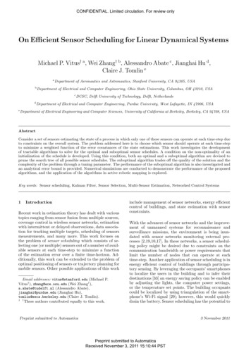
CONFIDENTIAL. Limited circulation. For review only ˆ(1)1 ˆ(1,1)2, 2(1,1), 1(1) 0 , 0 ˆ(1,2)2, 2(1,2) ˆCharacteristic set:3 (2,1)2, 2(2,1) ˆ 3 ˆ(2)1 , 1(2) ˆ , 3 : 3(2,2)2, 2(2,2) Fig. 1. The search tree and characteristic set for the sensor scheduling problem for an example with two sensors. This tree isthe enumeration of all possible sensor schedules with the corresponding covariance and running cost at each time-step. Thesuperscript for each covariance matrix, e.g. Σ̂(1,2) , denotes the sensor schedule used to obtain that estimate of the state.in Figure 1. Each node on the k th level of the tree corresponds to a k-horizon sensor schedule σ Mk and isrepresented by the so-called characteristic pair (Σσk , γkσ )that consists of the covariance matrix Σσk and the accrued cost γkσ Jk (σ) for the schedule σ. These pairscan be computed iteratively using the Riccati mapping.(1)(1)For example, the pair (Σ1 , γ1 ) in Figure 1 can be ob(1)(1)The main idea of the proposed solution method is motivated by the following properties of the Riccati mapping.Theorem 1 For any i M and any Σ1 , Σ2 A,(i) [Monotonicity] If Σ1 Σ2 , then ρi (Σ1 ) ρi (Σ2 );(ii) [Concavity] ρi (cΣ1 (1 c)Σ2 ) cρi (Σ1 ) (1 c)ρi (Σ2 ), c [0, 1].(1)tained as Σ1 ρ1 (Σ0 ), and γ1 tr Σ1 , whichcan in turn be used to compute the pair to its right (1,2)(1)(1,2)(1)(1,2)as Σ2 ρ2 Σ 1and γ2 γ1 tr Σ2.Clearly, if two nodes have the same characteristic pair,then they will have the same sets of descendants. Theset of all the characteristic pairs at time-step k is calledthe (k-horizon) characteristic set.Remark 1 The monotonicity property is a well-knownresult and its proof is provided in [16]. The concavityproperty is an immediate consequence of Lemma 1-(e)in [26].Thus, systems starting with a larger initial covariance,in the positive semidefinite sense, will yield larger covariances at all future time-steps. This result is importantbecause it provides insight on how to reduce the complexity of the scheduling problem.Definition 1 (Characteristic Set) The sequence ofNsets {Hk }k 0 generated recursively by Hk 1 hM (Hk )with initial condition H0 {(Σ0 , 0)} is called the characteristic set associated with Problem (5). Here themapping hM (·) is called the characteristic set mapping,which is defined by:Theorem 1 can be repeatedly applied to obtain the following corollary.Corollary 1 Let σ MN and Σ1 , Σ2 A, then k [0, N ], c [0, 1],(i) If Σ1 Σ2 , then φσk (Σ1 ) φσk (Σ2 );(ii) φσk (cΣ1 (1 c)Σ2 ) cφσk (Σ1 ) (1 c)φσk (Σ2 ).hM (H) {(ρi (Σ), γ tr(ρi (Σ))) : i M, (Σ, γ) H} .4The characteristic sets grow exponentially in size fromthe singleton {(Σ0 , 0)} to the set HN consisting of upto M N pairs, each comprising a positive semidefinitematrix and an accrued cost. Let Hk (i) (Σk (i), γk (i))be the ith element of the set Hk . For any subset Ĥk Hk ,the set of schedules corresponding to Ĥk is defined by,M(Ĥk ) {σ Mk : (Σ̂σk , γkσ ) Ĥk }.Computation of the Optimal Sensor ScheduleTo enable the study on larger systems with longerscheduling horizons, it is necessary to prune branchesfrom the exponential search tree that are redundant andthus will not lead to the optimal solution. The proposedalgorithm uses the properties of the Riccati mapping toobtain an easy-to-check condition to prune branches ofthe search tree without discarding the optimal schedule.(8)4Preprint submitted to AutomaticaReceived November 3, 2011 15:10:44 PST

CONFIDENTIAL. Limited circulation. For review only(1,2)(1,2)For example from Corollary 1, if two nodes (Σ̂2 , γ2(2,1)(2,1)and (Σ̂2 , γ2 ) in Figure 1 satisfy the condition(2,1)Σ̂2(1,2) Σ̂2(2,1)and γ2(1,2) γ2where r N t, s t 1 and l Ht . Finally, theconvex combination of the scalar variables indexed by iis lower bounded by the smallest one, i.e.,),γ then by the monotonicity of the Riccati mapping, all the(1,2)(1,2)descendants of the node (Σ̂2 , γ2 ) in the search treewill have a larger cost than the corresponding descen(2,1)(2,1)dants of the node (Σ̂2 , γ2 ). Hence, the exploration(1,2)(1,2)of the branches under (Σ̂2 , γ2 ) can be avoided, or(1,2)(1,2)equivalently the pair (Σ̂2 , γ2 ) can be pruned fromthe characteristic set H2 . Such a pair will be called redundant. By further considering the concavity of the Riccatimapping, other redundant pairs can be identified andpruned from the search tree. The following definitionprovides a condition to characterize redundant pairs.k s"Σ 0#0 γi 1l 1Xαi "Σ(i) 0i 10i [0,l 1] H {(Σ(i), γ(i))}i 1 , if the set H̄ H contains a schedulethat leads to the global optimal solution, i.e.min γ̄(i) min γ(i).i H̄ γ(i)Algorithm 1 [ES (H)]1: Sort H in ascending order such that γ(i) γ(i 1), i {1, . . . , H 1}2: H(1) {(H(1))}3: for i 2,. . ., H do4:if H(i) satisfies Definition 2 with respect to H(i 1)then5:H(i) H(i 1)6:else7:H(i) H(i 1) H(i)8:end if9: end forTheorem 2 If the pair (Σ, γ) Ht is algebraically redundant, then the pair and all of its descendants can bepruned without eliminating the optimal solution from thesearch tree.PROOF. Let (Σ, γ) be an algebraic redundant pairsatisfying the condition in Definition 2 with some conl 1stants {αi }i 1 . It suffices to show that there exists a pair Σ̃, γ̃ Ht \ (Σ, γ) such that σ N t MN t ,N t(Σ)) γ̃ k 1N tXtr(φσkN tAn efficient method for computing the optimal sensorschedule which uses the proposed pruning technique isstated in Algorithm 2. The procedure first initializes thecharacteristic set to the pair composed of the a prioricovariance of the initial state and initial cost. Then, foreach time-step it computes the characteristic set mapping and calculates the equivalent subset with Algorithm 1. Once the tree is fully built, the optimal sensorschedule is determined.(Σ̃)).k 1rFrom the monotonicity and concavity of φσk ,γ NXk srσtr(φk t(Σ)) l 1Xi 1"αii H According to Theorem 2 and Definition 3, an equivalentsubset of a characteristic set H can be obtained by removing all the redundant pairs in H as illustrated in Algorithm 1. The first step is to sort the set in ascendingorder based upon the current cost of the branches, whichis a reasonable heuristic for obtaining the minimum sizeof the equivalent subset. The equivalent subset is theninitialized to the current best branch. Next, each entryin H is tested with the current equivalent subset, H(i 1) ,to determine if it can be eliminated. If not, then it isappended to the current subset. The equivalent subsetreturned by this algorithm is denoted by ES (H).#Using Corollary 1, one can show that the branches corresponding to the redundant pairs can be pruned withoutdiscarding the optimal solution of the sensor schedulingproblem.tr(φσkk sDefinition 3 (Equivalent Subset) Let the set H̄ H̄ Σ̄(i), γ̄(i) i 1 be called an equivalent subset of H l 1N tXNXrtr(φσk t (Σ(i))). Thereforethe branch defined by (Σ, γ) and its descendants canbe eliminated because it will not contain the optimalsolution. 2where l H and {(Σ(i), γ(i))}i 1 is an enumeration ofH \ {(Σ, γ)}.γ k swhere i arg minγ(i) Definition 2 (Algebraic Redundancy) Apair(Σ, γ) H, where H is a characteristic set (Def. 1), iscalled algebraically redundant with respect to H\{(Σ, γ)},l 1if there exist nonnegative constants {αi }i 1 such thatl 1Xαi 1, andNNXXrrtr(φσk t (Σ)) γ(i ) tr(φσk t (Σ(i )))#NXrγ(i) tr(φσk t (Σ(i)))k s5Preprint submitted to AutomaticaReceived November 3, 2011 15:10:44 PST

CONFIDENTIAL. Limited circulation. For review onlyΣ1Algorithm 2 Sensor Scheduling for a Finite Horizon1: H0 {(Σ0 , 0)}2: for k 1,. . .,N do3:Hk hM (Hk 1 )4:Perform ES (Hk )5: end forσ6: σ arg min γNΣ̄ IΣ̃Σ2σ M(HN )Σ̄log(No. of branches)Number of Branches vs Time step60 1026Brute ForceExact Redundantε Redundant: ε 0.15040Fig. 3. Example covariances that demonstrate the concept of -redundancy. One possible convex combination of Σ1 and Σ2is represented by Σ̃ and let γ̃ be the same convex combinationof their costs. Σ1 and Σ2 cannot strictly eliminate Σ̄ becauseit does not contain Σ̃. However, if the condition is relaxedby , then Σ̄ I does contain Σ̃; consequently, if γ̄ γ̃then the branch can be eliminated.3020114 111000102030405Suboptimal Scheduling50Time step5.1Suboptimal Scheduling AlgorithmFig. 2. Comparison of the number of branches at eachtime-step for the brute force enumeration, the exact redundant elimination and the numerical redundant algorithm(See Section 5) with 0.1.To further reduce the complexity, the algebraic redundancy concept can be generalized to allow for numerical error. Similar to Definition 2, the following definitionprovides a condition for testing the -redundancy of amatrix.By using the proposed pruning technique, the complexity of the problem could be drastically reduced as displayed in the following example. Consider a system defined by Eqns. (1), (2) with three sensorsDefinition 4 ( -Redundancy) A pair (Σ, γ) H iscalled -redundant with respect to H \ {(Σ, γ)}, if therel 1exist nonnegative constants {αi }i 1 such that"A 0.9 0.15#",Σw 10l 1Xαi 1,#i 1,0.1 1.801hiC1 1.0 0.0 ,Σv1 0.1,hiC2 0.0 1.0 ,Σv2 0.3,hiC3 0.25 0.75 , Σv3 0.2,"Σ I00γ ##"l 1XΣ(i) 0 αi0 γ(i)i 1l 1where l H and {(Σ(i), γ(i))}i 1 is an enumeration ofH \ {(Σ, γ)}.Figure 3 illustrates the premise behind -redundancywith respect to Definition 4. Let Σ̃ represent one possible convex combination of Σ1 and Σ2 . In this example,Σ1 and Σ2 cannot strictly eliminate Σ̄ because Σ̄ doesnot contain Σ̃. However, if the condition is relaxed forsome 0, then Σ̄ I contains Σ̃. Consequently, forthat if γ̄ is greater than the same convex combination of γ1 and γ2 then Σ̄ can be eliminated. By using the -approximation it further reduces the numberof branches in the search tree and the complexity of theproblem. Consequently, this may enable the solution ofproblems that are otherwise intractable for the optimalalgorithm.and a schedule horizon of N 50. Figure 2 compares thenumber of branches required for the brute force enumeration versus Algorithm 2 which also provides the optimal solution but prunes redundant branches. At the finaltime-step, there are 1026 branches in the whole searchtree, but only 114 branches are required for Algorithm 2.Even though the optimal solution prunes a large number of branches, the growth of the search tree may stillbecome prohibitive for some problems. Therefore, an approximate solution may be desired.Similar to Algorithm 1, the convex condition in Definition 4 can be used to identify and prune -redundant matrices of a characteristic set. Denote by ES (H) the set6Preprint submitted to AutomaticaReceived November 3, 2011 15:10:44 PST

CONFIDENTIAL. Limited circulation. For review onlyof the remaining pairs after removing all the -redundantpairs in H that satisfy the conditions given in Definition 4. To determine the -approximate solution of thesensor scheduling problem, Algorithm 2 can be modified by substituting ES (·) for ES (·). The modified algorithm will be referred to as the suboptimal schedulingalgorithm (or ALGO ) in the rest of this paper. The essential part of this algorithm is to compute the so-calledN -relaxed characteristic sets {Hk }k 0 Hk ES (hM Hk 1), with H0 {(Σ0 , 0)} .To develop an analytical expression for the bound of theaverage-per-stage error, the effect of a perturbation ofthe initial covariance on all future covariances must bedetermined. To this end, the directional derivative of theRiccati mapping is first characterized.Lemma 1 For each i M and any Σ, Q A,dρi (Σ Q)d (9) Āi (Σ)QĀi (Σ)T , 0where Āi (Σ) is defined in Eqn. (11). The set HNtypically contains fewer pairs than HN andis easier to compute. To simplify the computation, theschedule that minimizes JN (σ) among all the schedules in M (HN) can be used as an alternative to the optimalschedule. Denote by σ ,N the suboptimal schedule computed by ALGO , namely,PROOF. Let i M, Σ A and Q A be arbitrarybut fixed. Define f ( ) Ci (Σ Q)CiT Σvi . It can beeasily shown that,df 1 ( ) f 1 ( )Ci QCiT f 1 ( ).d σ ,N arg min JN (σ).σ M(H N )Taking the derivative of ρi (Σ Q) with respect to andletting 0 yieldsAn example of the complexity for the suboptimal algorithm is shown in Figure 2 for an 0.1. By eliminating -redundant pairs, the complexity is reduced from114 for the optimal algorithm to 11. While the suboptimal algorithm drastically reduces the computationalcomplexity, it might sacrifice the quality of the solution.Consequently, an upper bound on the distance from theoptimal solution is needed.5.2dρi (Σ Q) AΣCiT f 1 (0)Ci QCiT f 1 (0)Ci ΣATd 0 AQAT AQCiT f 1 (0)Ci ΣAT AΣCiT f 1 (0)Ci QAT A (I ΣCiT f 1 (0)Ci )Q(I CiT f 1 (0)Ci Σ) AT . 1Noting that f 1 (0) Ci ΣCiT Σviand by the definition of Āi (Σ), the desired result is obtained. 2Performance AnalysisTheorem 3 For any Σ, Q A, i M and R , thefollowing holds:For each k N , define the (k-horizon) relaxed valuefunction Vk asVk min Jk (σ) σ M(Hk )min(Σ,γ) H kγ. ρi (Σ Q) ρi (Σ) Āi (Σ)QĀi (Σ)T .(10)Under this notation, the cost associated with the schedule returned by the suboptimal algorithm is VN . Thegoal of this section is to derive an upper bound for theaverage-per-stage error, namely N1 (VN VN ), incurredby the relaxation procedure of Eqn. (9).5.2.1PROOF. By the concavity of the Riccati mapping(Theorem 1), it can be easily verified that the mappingµi,Σ,Q : R A defined by µi,Σ,Q ( ) ρi (Σ Q), R , is also concave in for any i M. Thusµi,Σ,Q ( ) can be upper bounded by an affine functionof , namely, µi,Σ,Q (0) µ0i,Σ,Q (0) , which together withLemma 1 yields the desired inequality. 2Perturbation Analysis of the Riccati MappingFor each i M and Σ A, defineĀi (Σ) , A AKi (Σ)Ci ,(12)For any k 0, . . . , N , Σ A and σ MN , denote bygkσ (Σ; Q) the directional derivative of the k-step Riccatimapping φσk at Σ along an arbitrary direction Q A,i.e.,(11)where Ki (Σ) is the Kalman gain associated with sensori and matrix Σ defined asgkσ (Σ; Q) ,Ki (Σ) ΣCiT (Ci ΣCiT Σvi ) 1 .7Preprint submitted to AutomaticaReceived November 3, 2011 15:10:44 PSTdφσk (Σ Q)d . 0(13)

CONFIDENTIAL. Limited circulation. For review onlyTheorem 5 Fix arbitrary Σ A, N Z , and σ MN . If there exists a constant β such that Σσk (Σ) βIn for all k N , thenThe following lemma describes how to analytically compute gkσ , which will be useful in determining a bound forthe error incurred using the suboptimal algorithm.Lemma 2 For any Σ, Q A and σ MN , it holds thatg0σ (Σ; Q) Q andgkσ (Σ; Q) 0Qtr(gkσ (Σ)) where k 1 TQĀσ(t) (φσt (Σ)) QĀσ(t) (φσt (Σ)) ,t 0t k 1nβ kη , k 0, . . . , N,λ wη for k 1, . . . , N .1 11 αλ wandα λ w2kAk β 2 λ wβ. (14)Here, kAk denotes the Euclidean norm of A.PROOF. For simplicity, let Ât Āσ(t) (φσt (Σ)). Thecase k 0 follows directly from the fact thatPROOF. See Appendix.φσ0 (Σ Q) Σ Q.The above theorem reveals an important property of thek-horizon Riccati mapping φσk : A A, namely, boundedness of the trajectory implies an exponential disturbance attenuation. This property plays a crucial role inderiving the error boun

algorithms, and the application of the algorithms in active robotic mapping is explored. Key words: Sensor scheduling, Kalman Filter, Sensor Selection, Multi-Sensor Estimation, Networked Control Systems 1 Introduction Recent work in estimation theory has dealt with various topics ranging from sensor fusion from multiple sources,