WIXLIB

2017 IEEE International Symposium on Information Theory (ISIT)3when S(t1 ) S(t2 ) for any t1 , t2 . Moreover, A randomizedalgorithm specifies a probability distribution on the set of actions for each decision epoch, while a deterministic algorithmchooses an action with certainty.The long-run average cost for some history dependentalgorithm θ is given by T 1V (θ) lim supEθC(S(t), D(t)) S(0) ,T T 1t 0where Eθ represents the conditional expectation, given thatthe policy θ is employed.Definition 1. A scheduling algorithm θ is average-optimal ifit minimizes the long-run average cost V (θ).Our goal is to characterize and obtain an average-optimalalgorithm. However, according to [12], there may not exist astationary or deterministic algorithm that is average-optimalfor an infinite state-space MDP. Due to the space limitation,we present our main results in this paper, and please see ourtechnical report in [11] for the complete proofs.III. C HARACTERIZATIONS OF THE AVERAGE - OPTIMALITYWe begin with an infinite horizon α-discounted cost case,where 0 α 1; we then tie to the average cost case becausestructures of the average-optimal algorithm usually rely on thediscounted cost case. Given initial state S(0) s, the totalexpected discounted cost under an algorithm θ is T tVα (s; θ) lim Eθα C(S(t), D(t)) S(0) s .T t 0Definition 2. A scheduling algorithm θ is α-optimal if itminimizes the total expected discounted cost Vα (s; θ). Inparticular, we defineVα (s) min Vα (s; θ).θWe first introduce the discounted cost optimality equationfor Vα (s) as below.Proposition 3. The optimal expected discounted cost Vα (s),for state s, satisfies the following discounted cost optimalityequation:Vα (s) mind {0,1,··· ,N }C(s, d) αE[Vα (s )],(1)where the expectation is taken over all possible next state s reachable from the state s. A deterministic stationary algorithm that realizes the minimum of the right hand side (RHS)of the discounted cost optimality equation will be an α-optimalalgorithm. Moreover, we define Vα,n (s) by Vα,0 (s) 0 andfor any n 0Vα,n 1 (s) mind {0,1,··· ,N }C(s, d) αE[Vα,n (s )].(2)Then, Vα,n (s) Vα (s) as n for every s, and α.Proof. (Sketch) Basically, we need to verify that Vα (s) is finitefor all possible α and s. Please see [11] for details.Lemma 4. There exists a deterministic stationary algorithmthat is average-optimal. Moreover, there exists a finite constantg limα 1 (1 α)Vα (s) for every state s such that theaverage-optimal cost is g, independent of the initial state S(0).Proof. Please see [11].We remark that even though the average-optimality of adeterministic stationary algorithm is shown in Lemma 4, wemight not arrive at an average cost optimaility equation likeEq. (1) or the value iteration like Eq. (2) (see [13, 14] fordetails).In addition to the average-optimality of a deterministic stationary algorithm, we show that an average-optimal schedulingalgorithm has a nice structure facilitating the scheduling algorithm design in the next section.Definition 5. A switch-type algorithm is a deterministic stationary algorithm: for every user ui , if an average-optimaldecision for state s (a1 , · · · , ai , · · · , aN , λ1 , · · · , λN ) isd s i, then an optimal decision at state s (a1 , · · · , ai 1, · · · , aN , λ1 , · · · , λN ) is d s i as well.Theorem 6. An average-optimal scheduling algorithm is theswitch-type algorithm.Proof. (Sketch) We first prove that an α-optimal schedulingalgorithm is the switch-type by applying the value iteration inEq. (2). Then, we show that the structure holds for the averageoptimum by letting α 1. Please see [11] for details.In particular, if the arrival rates of all information sourcesare the same, we can obtain a nice index algorithm as follows.Corollary 7. If the arrival rates of all information sourcesare the same, i.e., pi pj for all i j, then an optimalscheduling algorithm updates the user with the largest age,i.e., D(t) arg maxi Ai (t) for each time t.Proof. Please see [11].We also notice that the index algorithm is indeed an on-linealgorithm, without the knowledge of the arrival statistics inadvance. For general asymmetric arrivals, an average-optimalscheduling algorithm depends on both the arrival statistics andthe current ages. However, it is not obvious how to get anaverage-optimal scheduling for the asymmetric arrivals. Thiskey challenge hence motivates us to investigate both off-lineand on-line scheduling algorithms in the next section.IV. S CHEDULING ALGORITHM DESIGNWe start with proposing finite-state approximations to theoriginal MDP as in practice we can only work on a finitestate MDP to avoid formidably high computation complexity.We will rigorously show the convergence of the proposedtruncation as in general a MDP truncation might not convergeto the original MDP according to [14].Based on the finite-state MDPs, we first propose a structuralvalue iteration algorithm in Section IV-B to pre-compute anoptimal decision for each state, whose complexity wouldbe lower than the conventional value iteration algorithm byemploying the switch structure. Moreover, we propose an online algorithm leveraging the stochastic approximation [15] inSection IV-C563

2017 IEEE International Symposium on Information Theory (ISIT)4A. Finite-state MDP approximationsAlgorithm 1: Structural off-line scheduling algorithmLet Δ be the Markov decision process defined in Section II-B. By {Δm } we define a sequence of approximateMDPs for Δ whose state-space is Sm {s S : ai m}with the bounded virtual ages, while the decision-space andcost definition are the same as Δ.(m)Let Ai (t) be the age of information for user ui at time tfor Δm . Different from Δ, under decision D(t) d the age(m)(m)of the next slot for Δm is Ad (t 1) 1 and Ai (t 1) (m) if i d, where we define the notation [x] Ai (t) 1mm by [x] m x if x m and [x]m m if x m.(m)Let Ps,s (d) be the transition probability for Δm . Then,(m)Ps,s (d) Ps,s (d) if s Sm ; otherwise, (m)Ps,r (d),Ps,s (d) Ps,s (d) r S Smfor some excess probabilities on state r S Sm .Next, we show that the proposed finite-state approximationswill be asymptotically average-optimal.Theorem 8. Let V and Vm be the average-optimal cost toΔ and Δm , respectively. Then, Vm V as m .Proof. Please see [11].Now, we are ready to propose scheduling algorithms basedon Δm . In other words, the BS make decisions according to(m)the virtual age Ai (t) on Sm , instead of the real age Ai (t)on S. The real age can increase beyond m but the virtual agewill be smaller than m 1.B. Structural off-line scheduling algorithmThe relative value iteration algorithm (RVIA), as follows,can be applied to get an optimal deterministic stationaryalgorithm on Δm :Vn 1 (s) mind {0,1,··· ,N }C(s, d) E[Vn (s )] Vn (0),(3)for all s Sm , where 0 is a reference state and we can arbitrarily choose the reference state by 0 (1, 2, · · · , N, 1, · · · , 1).For each iteration n, we need to update the decisions for allvirtual states by minimizing the RHS of Eq. (3) as well asupdate V (s) for all s Sm . The complexity is very high dueto many users (i.e., curse of dimensionality [16]). Therefore,we propose in Alg. 1 a structural off-line algorithm based onthe RVIA along with the switch structure.In Alg. 1, we seek an optimal decision d s for each virtualstate s Sm by iteration. For each iteration, we update bothoptimal decision d s and V (s) for all virtual states. If theswitch property holds, we can determine an optimal decisionimmediately in Line 5; otherwise we find an optimal decisionaccording to Line 7. By Vtmp (s) in Line 9 we temporarilykeep the updated value, which will replace V (s) in Line 11.Using the switch structure to prevent from the minimumoperations on all virtual states in the RVIA, we can reducethe computational complexity accordingly. We conclude theoptimality of Alg. 1 in the following.123456789101112V (s) 0 for all states s Sm ;while 1 doforall s (a1 , · · · , ai , · · · , aN , λ1 , · · · , λN ) Sm doif there exists ζ 0 and i {1, · · · , N } such thatd (a ,··· ,a ζ,··· ,a ,λ ,··· ,λ ) i then11iNNd s i;elsed s arg mind {0,1,··· ,N } C(s, d) E[V (s )];endVtmp (s) C(s, d s ) E[V (s )] V (0);endV (s) Vtmp (s) for all s Sm .endTheorem 9. The limit point of d s of Alg. 1 is an averageoptimal decision for all virtual state s Sm . In particular,Alg. 1 converges in a finite number of iterations.Proof. (Sketch) We need to verify that the finite-state approximate MDPs are unichain. Please see [11] for details.C. On-line scheduling algorithmWe notice that Alg. 1 needs the arrival statistics to precompute an optimal decision for each virtual state. We willpropose an on-line scheduling algorithm in case that thestatistics is unavailable. Instead of updating V (s) for all statesat each iteration, we update V (s) following a sample path,which is a set of outcomes of the arrivals over slots. It turnsout that the sample-path updates will converge to the averageoptimal solution.To that end, we need a stochastic version of the RVIA.However, the RVIA in Eq. (3) is not suitable because theexpectation is inside the minimization (see [16] for details).Moreover, minimizing the RHS of Eq. (3) for a given currentstate needs the transition probabilities to calculate the expectation. To tackle these challenges, we design post-decisionstates [16] for our problem.We define the post-decision state s̃ as the ages andthe arrivals after a decision. The state we used before is referred to as the pre-decision state. If s (a1 , · · · , aN , λ1 , · · · , λN ) Sm is a virtual state of thesystem, then the virtual post-decision state after decision dis s̃ (ã1 , · · · , ãN , λ̃1 , · · · , λ N ), where ãi 1 if i d and ãi [ai 1]m otherwise, as well as λ̃i λi for all i.Let Ṽ (s̃) be a value function based on the post-decisionstates:Ṽ (s̃) Es [V (s)],where the expectation Es is taken over all the predecision states reached from the post-decision state. Wecan then write down the post-decision average cost optimality equation [16] for the virtual post-decision age s̃ (ã1 , · · · , ãN , λ̃1 , · · · , λ̃N ) with s̃ Sm :564Ṽ (s̃) g Emind {0,1,··· ,N } C (ã, λ̃ ), d Ṽ ([ã 1 ãd ] m , λ̃ ) ,

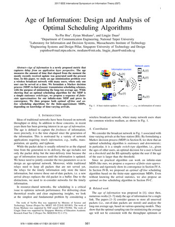
2017 IEEE International Symposium on Information Theory (ISIT)52345D (t) arg mind {0,1,··· ,N } Ṽ ([ã 1 78910(5)where ãi (0, · · · , ãi , · · · , 0) is the zero vector except forthe i-th entry being substituted by ãi , and 1 (1, · · · , 1) isthe unit vector. Moreover, λ̃ is the next possible arrivals.From above optimality equation, the RVIA is as follows:Ṽn 1 (s̃) Emind {0,1,··· ,N }C (ã, λ̃ ), d Ṽn ([ã 1 Ṽn (0). ad ] m , λ̃ ) (4)Then, we are ready to propose the on-line algorithm inAlg. 2 based on a stochastic version of the RVIA. In Lines 1-3,we initialize Ṽ (s̃) of all virtual post-decision states and startfrom the reference point. Moreover, by v we record Ṽ (s̃) ofthe current virtual post-decision state.By observing the current arrivals Λ(t) and plugging inEq. (4), in Line 5 we optimally update a user by minimizingEq. (5); as such, the expectation in Eq. (4) is removed. Then,we update Ṽ (s̃) of the current virtual post-decision state inLine 7, where γ(t) is a stochastic step-size (see [16]) at slott and hence Ṽ (s̃) is balanced between the previous Ṽ (s̃) andthe current value v. Finally, the next virtual post-decision stateis updated in Lines 8 and 9. Theorem 10. If t γ(t) and t γ 2 (t) , then Alg. 2converges to the average-optimal value.Proof. Please see [11].43.5On line algorithmOff line algorithm111098760.40.50.60.70.8Arrival rate (p)0.90.40.50.60.70.8Arrival rate (p)0.9Fig. 2. The average total age over 100,000 slots versus the symmetric arrivals(i.e., pi p for all user ui ) by employing Algs. 1 and 2 for two users (leftfigure) and three users (right figure).end 54.52.5/* Value update */v C ((ã, Λ(t)), D (t)) Ṽ ([ã 1 ãD (t) ] m , Λ(t)) Ṽ (0);Ṽ (s̃) (1 γ(t))Ṽ (s̃) γ(t)v;/* Post-decision state update */ã [ã 1 ãD (t) ] m;λ̃ Λ(t).65.53C ((ã, Λ(t)), d)ãd ] m , Λ(t));On line algorithmOff line algorithm6Average total age16.5/* Initialization */Ṽ (s̃) 0 for all states s̃ Sm ;s̃ 0;v 0;while 1 do/* Decision at slot t */We optimally make a decision D (t) at slot t according to thecurrent arrivals Λ(t) (Λ1 (t), · · · , ΛN (t) at slot t:Average total ageAlgorithm 2: On-line scheduling algorithm In the above theorem,t γ(t) implies that Alg. 2needs infinite number of iterations to learn the average-optimalsolution, while Alg. 1 can converge to the optimal solution ina finite number of iterations. Moreover, t γ 2 (t) meansthat the noise from measuring Ṽ (s̃) can be controlled.Finally, we want to emphasize that the proposed Algs. 1 and2 are asymptotically optimal, i.e., they converge to the optimalsolutions when the finite state-space m and the slots t go toinfinity. In Fig. 2, we show the performance of Algs. 1 and 2over finite slots. In our technical report [11], we provide morenumerical studies and discussions of the proposed algorithmsfor both no-buffer network and buffer-network.V. C ONCLUSIONIn this paper, we consider a broadcast network, wheremany users are interested in different information that shouldbe delivered by a base-station. We theoretically investigatethe long-run average age of information by designing andanalyzing optimal scheduling algorithms. We show that anoptimal scheduling algorithm is a simple stationary switchtype. To tackle the infinite state-space Markov decision process(MDP), we propose a sequence of finite-state approximateMDPs. Based on the approximate MDPs, we propose bothoff-line and on-line scheduling algorithms. It turns out theproposed algorithms are asymptotically optimal.R EFERENCES[1] S. Kaul, R. D. Yates, and M. Gruteser, “Real-Time Status: How OftenShould One Update?” Proc of IEEE INFOCOM, pp. 2731–2735, 2012.[2] C. Kam, S. Kompella, G. D. Nguyen, and A. Ephremides, “Effect ofMessage Transmission Path Diversity on Status Age,” IEEE Trans. Inf.Theory, vol. 62, no. 3, pp. 1360–1374, 2016.[3] L. Huang and E. Modiano, “Optimizing Age-of-Information in a MultiClass Queueing System,” Proc. of IEEE ISIT, pp. 1681–1685, 2015.[4] Y. Sun, E. Uysal-Biyikoglu, R. D. Yates, C. E. Koksal, and N. B.Shroff, “Update or Wait: How to Keep Your Data Fresh,” Proc. of IEEEINFOCOM, pp. 1–9, 2016.[5] R. D. Yates, “Lazy is Timely: Status Updates by an Energy HarvestingSource,” Proc. of IEEE ISIT, pp. 3008–3012, 2015.[6] B. T. Bacinoglu, E. T. Ceran, and E. Uysal-Biyikoglu, “Age of Information under Energy Replenishment Constraints,” Proc. of ITA, pp. 25–31,2015.[7] M. Costa, M. Codreanu, and A. Ephremides, “On the Age of Informationin Status Update Systems with Packet Management,” IEEE Trans. Inf.Theory, vol. 62, no. 4, pp. 1897–1910, 2016.[8] L. Golab, T. Johnson, and V. Shkapenyuk, “Scalable Scheduling ofUpdates in Streaming Data Warehouses,” IEEE Trans. Knowl. Data Eng.,vol. 24, no. 6, pp. 1092–1105, 2012.[9] Q. He, D. Yuan, and A. Ephremides, “Optimizing Freshness of Information: On Minimum Age Link Scheduling in Wireless Systems,” Proc.of WiOpt, pp. 1–8, 2016.[10] I. Kadota, E. Uysal-Biyikoglu, R. Singh, and E. Modiano, “MinimizingAge of Information in Broadcast Wireless Networks,” Proc. of Allerton,2016.[11] Y.-P. Hsu, E. Modiano, and L. Duan, “Age of Information: Design andAnalysis of Optimal Scheduling Algorithms,” Technical report, 2017.[Online]. Available: http://web.ntpu.edu.tw/%7Eyupinhsu/age.pdf[12] M. L. Puterman, Markov Decision Processes: Discrete Stochastic Dynamic Programming. The MIT Press, 1994.[13] L. I. Sennott, “Average Cost Optimal Stationary Policies in InfiniteState Markov Decision Processes with Unbounded Costs,” OperationsResearch, vol. 37, pp. 626–633, 1989.[14] ——, Stochastic Dynamic Programming and the Control of QueueingSystems. John Wiley & Sons, 1998.[15] V. S. Borkar, Stochastic Approximation: A Dynamical Systems Viewpoint. Cambridge University Press, 2008.[16] W. B. Powell, Approximate Dynamic Programming: Solving the Cursesof Dimensionality. John Wiley & Sons, 2011.565

algorithms for minimizing the average age. The model in [7] uses a small buffer to store the latest information. Of the most relevant work to us about scheduling for multiple users is [8-10]. Both [8, 9] consider queues at a BS, while [8] develops some hueristic scheduling algorithms and [9] analyzes the complexity of scheduling for .