Transcription
A Data Warehouse System for Estimating FuelConsumption from Multiple Traffic Data SourcesRune Bak Jacobsenrbja16@student.aau.dkAalborg UniversitetSøren Andreas Abildskov Hansensaah16@student.aau.dkAalborg Universitetfrom stationary measurement stations, consisting of data frompoints, which are a set of latitude and longitude coordinates.The data in the FCDD is obtained from GPS devices invehicles given from road segments as a stretch of road.Additionally, we use OpenStreetMaps (OSM) as a commonrepresentation. Separated, these data sources cannot representthe density of the traffic in a traffic network. However, thestrengths of the data sources cancel out the weaknesses ofthe opposite source. Thus, we integrate the data sources intoa common representation. However, as the data sources havedifferent spatial and temporal representations, the integration isnot straightforward. It includes, among others, map matchingof ILDD and FCDD to OSM road segments. Section 6describes the entire data integration process. The FCDD andILDD register the Annual Average Daily Traffic [3] (AADT),which is the yearly number of vehicles on a given road.Throughout this paper, the AADT will be referred to as hitsfor a given road segment. The FCDD and ILDD also registerthe average speed.However, the FCDD does not register the total density oftraffic on its road segments as it only registers a subset ofall vehicles. This is due to the data being vehicle dependentand not location dependent. Likewise, ILDD does not capturethe entire traffic flow since it registers data from stationarystations located at specific points. Unfortunately, not everyroad segment has a measurement station, as the deploymentmaintenance of such stations is costly. Thus, stations registercomplete data, but their coverage of a road network is sparse.In order to extrapolate the hits from the FCDD to the completehits number given from the ILDD, we use linear regression.The approach creates a model which can predict the ILDDhits value given an FCDD hits value. Additionally, a modelto predict the ILDD average speed given the FCDD averagespeed us also used. When the data integration of the sources iscomplete, we utilize a fuel estimation model to estimate fuelconsumption on road segments. The fuel estimation modeltakes different vehicle parameters as input, capturing thevariations among vehicles and affecting fuel consumption. Asan example, a small car usually uses less fuel than a large car,and a truck uses more fuel than a large car. For that reason,the system supports creating custom vehicle types. This worksby specifying the parameters of the given vehicle to be usedin the fuel estimation model. The vehicle parameters include,e.g., the weight of the vehicle and the idle fuel consumption.Furthermore, one can specify the vehicle distribution ofAbstract—Given the need to reduce greenhouse gas emissionsthroughout society, methods are needed to estimate current emissions reliably so that the effects of initiatives towards reducingemissions can be assessed. This paper focuses on traffic and how,given traffic data, we can provide insight into the total emissionsof the municipality. The data sources are Induction Loop DerivedData and Floating Car Derived Data. A data warehouse design isproposed, and the paper elaborates on the benefits of the design.A fuel estimation model uses the processed traffic data to estimatefuel consumption and CO2 emissions.Furthermore, the model uses custom vehicle sets to reflectthe real-life traffic of a municipality. The paper offers insightinto the strengths and weaknesses of the approach and exploresalternative methods for modifying and improving the approach.The system provides estimations for fuel consumption and CO2from spatial and temporal queries through an interface.1. I NTRODUCTIONA. MotivationOn December 12, 2015, 196 parties to the UN adoptedThe Paris Agreement [1]. The agreement’s goal is to limitgreenhouse gas emissions to slow global warming. Subsequently, Danish municipalities created the ”DK2020” [2] plan,which represents the commitment to reaching the goals definedin The Paris Agreement. Currently, 66 out of 98 Danishmunicipalities have joined the plan. The plan centers around acollaborative effort where the municipalities can share experiences and solutions to create a framework to prevent climatechange. With the growing commitment to reduce greenhousegas emissions, it is necessary to create new solutions thatsupport this development.In Europe, out of the total CO2 emissions, nearly 30%comes from traffic, of which 72% is from road traffic. Thus, alarge part of greenhouse emissions comes from traffic. Thispaper studies how to provide fuel consumption and CO2emission estimates given two different sources of traffic data.Thus, the solution gives insight into the current situation andplan for future scenarios regarding fuel consumption and CO2emission estimates.B. ContributionsThis paper introduces a system to compute fuel estimationsof vehicles traveling in a road network from two traffic datasources. As fuel and CO2 emissions are proportional to eachother, the paper focuses on fuel estimations. The traffic datasources are Induction Loop Derived Data (ILDD) and FloatingCar Derived Data (FCDD). The data in the ILDD is obtained1
trucks, buses, and cars. This allows analyzing different scenarios such as traffic with or without electric buses. Thus, it ispossible to see how fuel usage will decline as electric vehiclesincrease. The results of the system are accessible in a webapplication. The application takes a temporal input in the formof a number of days and a time period. Thus, it is possible tospecify the time period, e.g., between 15.00 and 16.00, downto a 15-minute range. The web application also contains a mapfrom which the users can draw polygons to query on the roadnetwork. This usage enables, e.g., investigation of fuel usagein a city versus on motorways. Appendix A shows an exampleof the result page from the web application.approach as we also will use a linear regression model. Wetake a different approach for this paper as we use a secondAADT measurements source for the model instead of variablessurrounding the roads.In ”An Advanced Data Warehouse for Integrating LargeSets of GPS Data” [6], they implemented data warehouses forGPS data using PostgreSQL [7] with the PostGIS [8] extension. For the ETL flow, they used a programmatic approachusing pygrametl, which ”pygrametl - ETL programming inPython” [9] and ”Programmatic ETL” [10] documents. Wewill use PostgreSQL with the PostGIS extension for the datawarehouse and pygrametl for the ETL process for this paper.3. U SE C ASESC. OverviewAs described in Section 1-A, the paper aims to aid Danishmunicipalities in estimating traffic fuel usage. In order toget an understanding of the use cases, we cooperated witha Danish consultant company which specializes in trafficdata solution for the Danish municipalities. The usage of thesystem is intended to be made available by said company tothe Danish municipalities.The paper first covers the related works in Section 2. Next,Section 3 describes the use cases of the system. Followingthis, Section 4 explains the system flow. Here we give anoverview of the functionality of the entire system. Section 5describes the used fuel estimation model SIDRA-RUNNING.We go through which parameters are necessary for the modelto function and support vehicle sets. Section 6 explains the datasources and integration and covers the steps from raw data to acommon representation. Section 7 explains the data warehousearchitecture. Section 8 looks at linear regression models to predict accurate hit numbers and accurate average speed numbers.Section 9 reiterates our use cases and showcases the results.Following this, Section 10 will discuss the decisions throughout the paper and the processes leading to the final results.Finally, Section 11 will summarize and conclude the paper.A. Yearly EstimateOne of the primary requests is to get a yearly estimateof the fuel consumed and CO2 emitted in a user-specifiedgeographical region. This is the primary feature, and thus thesystem needs to present this properly. The feature considersmultiple traffic states with free-flowing traffic and spike hours,based on our data sources. Another aspect is to distinguishweekdays and weekends as the total traffic will be different.Thus, we must calculate the yearly total estimate accordingly.2. R ELATED W ORKEcoMark 2.0 [4] studies multiple fuel estimation modelsto compare their results to ground truth data measured fromvehicles. The paper tests both instantaneous and aggregatedfuel models, where instantaneous models use point data andaggregated models use road segment data. As for relevance tothis paper, they concluded that the SIDRA-RUNNING modelwas suitable for assigning eco-weights to road segments, thusmaking the model viable for fuel consumption estimations.They also used the SIDRA-Avg model, but the model doesnot apply to all road categories, as it becomes unreliablewhen the average speed excels 50 km/h. For this paper, weuse the fuel model SIDRA-RUNNING based on the resultsfrom EcoMark 2.0.”Estimating traffic volume on Wyoming low volume roadsusing linear and logistic regression methods” [5] describesa method to try and estimate the AADT traffic densitymeasurement on low-volume roads in Wyoming using linearand logistic regression. The intended usage of the methodwas for low-volume rural roads. The study used linear andlogistic regression to try and give an estimate based on severalpredictor variables, which include, e.g., the surface of theroads and the population near the roads. They found thatland usage near the roads was the most significant predictorvariable. Their model scored an R2 value varying from 0.44up to the best score of 0.64. For this paper, we use a similarB. Estimate ScalingIn addition to the yearly estimate, the yearly developmentof the total emissions is also relevant to investigate. As thenumber of vehicles increases in municipalities, the total fueland CO2 will also increase. Thus, a parameter to alter thetotal number of vehicles can provide additional informationfor future scenarios.C. Vehicle SetsFinally, an aspect that affects the total fuel used is the typeof vehicles driving in the municipalities. If the vehicles areprimarily gas and diesel vehicles, the total fuel used will begreater than a scenario where a subset of the vehicles areelectric vehicles. The ability to model an increase in electricvehicles means seeing how electric vehicles impact the totalfuel and CO2 usage.4. S YSTEM D ESIGN & F LOWWe created the system as a web application, from which allthe functionality is available. To be specific, the functionalitymanages the traffic data upload, applies the fuel estimationmodel with different parameter sets, and presents the results.Figure 1 shows the flow of the system.The center column consists of the three main pages,Upload, Parameters, and Cases, and the ETL flow. Each of2
road segment data. Another option was the SIDRA-AVERAGEmodel, which also uses segment data. However, the originalpaper [11] declared the model unfit to estimate fuel whenthe average speed exceeds 50 km/h. Furthermore, since thetraffic data concerns both rural and urban driving, the model isnot viable. Based on SIDRA-RUNNING’s features and giventhe inapplicability of SIDRA-AVERAGE, we use SIDRARUNNING as the fuel estimation model.A. Model DescriptionThe SIDRA-RUNNING model uses variables regarding aroad segment and a vehicle to estimate the fuel required totraverse that given road segment with the given vehicle. For aroad segment, the model uses the variables listed below fromthe input data. However, the model uses additional variablesnot available from the data. Thus, they are estimated based onthe calculations from the original paper [11]. To summarize,the variables we use from our data sets are the following two. Average speed Total segment distanceIn addition to the driving behavior variables, the SIDRARUNNING model also uses vehicle-specific parameters, asthere is a difference between the fuel usage among vehicles,e.g., a heavy truck uses more fuel than a small car. In orderto accurately provide fuel estimations that also account forvehicle diversity, we are taking two approaches. First, we usethe vehicle set defined by Akçelik et al. in [12]. This setcontains three car types, one bus type and one truck type,which were created and calibrated by the authors of the SIDRAmodels. Additionally, we include an electric vehicle type witha fuel usage of 0 to take into account the growing percentage ofelectric vehicles. Second, we support custom vehicle creationby the users of our system to accommodate for the evolutionof vehicles, e.g., vehicles driving farther using less fuel. Theresult of the model is an estimate of the fuel consumed on aroad segment given in mL. To get the CO2 emitted, the fuelestimate is multiplied by 2.29 for gas or 2.66 for diesel [13].The SIDRA-RUNNING model is given as:(α ti fr xs f or 0 fr xsFs α tiotherwiseFig. 1: System flowthem has their process flow mapped through the roundedrectangles following their small arrow. The system startsfrom the Upload page, where the users upload the FCDD andILDD. The ETL flow then processes the data and integrates itinto a common source. The ETL process is described furtherin Section 6 and Section 8.When the ETL flow is complete, the user can, through theParameters page, create custom parameter sets and apply themto the uploaded data. A parameter set contains a vehicle growthparameter which is a percentage indicator to scale the totalnumber of vehicles from the uploaded traffic data. A parameterset also contains a vehicle set that represents the vehiclespresent in the road network. Furthermore, the user can specifyvehicle sets, giving complete control of which vehicles toapply to the traffic data and the percentage each vehicle shouldrepresent. It is possible to apply many parameter sets to thesame uploaded data, enabling comparison between multiplemodels of the data.After applying the chosen parameter sets, the user can goto the Cases page to view the results. The Cases page allowsthe user to input an upload name, an applied parameter set,a time period, a number of days, and a polygon. Then, thesystem returns the fuel consumption for the area in the giventime period. The user creates polygons using Leaflet1 , a librarythat allows the user to draw a polygon point by point. The usercan then compare different model results from the uploadedtraffic data. Appendix D shows the different functionality ofthe web application.fr fi /vr A Bvr2 Q1 Q2 0.0981KG β1 M GQ1 KE1 β1 M Ek 2Q2 KE2 β2 M Ek (0.675 1.22/vrKE1 0.55. S IDRATo provide fuel estimates based on the data sources, weuse a model that utilizes the data features. As mentionedin Section 2, Eco-Mark-2.0 tested several fuel estimationmodels to determine how closely they compared to groundtruth fuel data. One of the methods used was the SIDRARUNNING model, which showed promising results based onf or 0.5 0.675 1.22/vrotherwiseKE2 2.78 0.0178vr(1 1.33EK f or G 0KG 0.9otherwise(0.35 0.0025vr f or 0.15 0.35 0.0025vrEK 0.15otherwise(1)1 https://leafletjs.com3
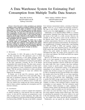
In the model, Fs is the fuel consumed in mL, fr is the fuelconsumption in mL/km, xs is the segment length in km, vris the travel speed in km/h, ts is the travel time in seconds,ti is the idle time in seconds, EK is the sum of positivekinetic energy changes per unit mass per unit distance, and Gis the road grade. The parameters fi , α, A, B, β1 , β2 , andM are vehicle parameters, and lastly KE1 , KE2 , and KG arecalibration parameters. The complete model can be found inthe literature [11].stations, and the FCDD road network is composed of 58.484road segments.B. OpenStreetMapsTo combine FCDD and ILDD to a common representation,we use OpenStreetMaps’ road network (OSM). The roadnetwork consists of a number of road segments. The roadsegments can vary in length and structure. Figure 2 showsan example with five segments where a single blue line witha black border represents a road segment.B. Vehicle SetsWhen using SIDRA-RUNNING, many of the variables arevehicle specific, and thus the result becomes vehicle specific.As there is a wide variety in the type of vehicles in everydaytraffic, the system must account for this. To accomplish this, itis possible to create custom vehicles with the parameters specified. This allows for custom vehicle sets creation consisting ofa set of vehicles and the percentage each vehicle makes of thefull set. Currently, the vehicles separate into three categories;cars, buses, and trucks. The reason is to be able to distinguishdifferent vehicle types from each other. It is also possible tocreate electric vehicle types to reflect the number of electricvehicles currently driving, which do not consume fuel such aspetrol or diesel. For this paper, we do not consider the electricenergy for electric cars in terms of CO2 output.6. DATAA. OverviewFig. 2: OpenStreetMaps road segmentsAs mentioned in Section 1-B, the paper uses the trafficdata sources FCDD and ILDD and uses a map representationfrom OSM. Since FCDD uses a proprietary map and ILDDonly provides coordinates of its stations, we use OSM’s roadnetwork to connect them.The traffic information from FCDD and ILDD are contrasting. The FCDD consists of traffic data for many roadsegments, which, when combined, creates a road network.In this regard, the data is complete. However, the registeredtraffic data in FCDD is sparse, as it does not reflect everyvehicle that has been in the road network. This is becausethe registrations are from, e.g., navigation systems. ILDDonly provides the specific point for each measurement station.These are stationary and registers the total traffic at a giventime in a specific place. The traffic data from ILDD is thencomplete as it registers all vehicles at a specific point. Inregards to a road network, it is a sparse data source sincethere are only a limited number of stations. Appendix B givesan overview of the FCDD road segments and the ILDD points.Both FCDD and ILDD support varying time granularity,with the finest being 15-minute intervals. The system proposedin this paper supports these temporal representations. Thissection describes how we integrate the finest time granularityas it requires additional processing. Furthermore, it enablesthe system to make more fine-grained temporal queries.The data used for this paper is from February 2019 to February 2020 for Odense municipality. The time granularity is 15minute intervals. The ILDD is composed of 85 measurementThe road segments in OSM also have associated metadata.Table 1 shows an example of the information used from OSM.Id121390376NameSkovalléenHighwaytertiaryMax Speed50Table 1: Example of OSM road segmentC. Floating Car Derived DataAs mentioned, the FCDD provides traffic data assigned toroad segments. Since there are different ways to model roadnetworks, the road segments can vary in length. This is thecase with the FCDD road network compared to the OSMroad network. To illustrate, Figure 3 shows the same streetwith road segments from the FCDD. The road segments havea black border to indicate where they begin and end. Asmentioned, there are a total of 58.484 road segments for theFCDD road network.Table 2 shows an example of the traffic data associated witha road segment. Hits is the number of vehicles registered forthe road segment in the time period, AvgSp is the averagespeed in km/h of the vehicles, and AvgTt is the average traveltime in meSkovalléenAvgSp AvgTt33,553,82Hits201Table 2: Example of FCDD row, weekday during 11.45–12.004
number of vehicles and their average speed. Table 3 shows anexample of ion01.02.2019 -Count57Speed34,1Table 3: Example of ILDD row, 01.02.2019 during 11.45–12.00Contrary to FCDD, ILDD contains dates, which means thereare rows for every day of the year, with 15-minute intervalsassociated with it.E. Data IntegrationBoth FCDD and ILDD have their strengths and weaknesses.The goal is to integrate the two sources into a single soliddata source. This integration includes the date representation inILDD and the lack of it in FCDD. Also, the integration correctsthe spatial representations to a common representation.The data integration integrates FCDD, ILDD, and OSM intoa unified format. Furthermore, the resulting rows capture thecombined data of the road segments. The process is three steps.One step for the ILDD, one step for the FCDD, and the laststep is merging the two.1) ILDD Transformation: Each measurement station registers independent data from the other. For that reason, weperform the transformation for every station. Since we wantto integrate the ILDD and the FCDD, we group the individualdates to reach the same aggregation. This works by settingthe date as a weekday or a weekend day. Following that, it ispossible to group the measurement station based on if it is aweekday or not.Example: Table 4 shows four rows from the measurementstation on Skovalléen during 11.45–12.00. Depending on thedate of the measurement, a weekday flag determines whetherit is a weekday or weekend day. We omit the coordinates ofthe measurement stations for brevity.Fig. 3: FCDD Segments ExampleThis paper uses the data in 15-minute intervals, e.g., from11.45–12.00, and in two periods. The first period is Tuesdays,Wednesdays, and Thursdays to represent a weekday, and thesecond period is Saturdays to represent a weekend day. Noticethat the FCDD does not have a date specified with it. This isdue to the data is aggregated. This means that the vehiclesregistered in a time period are for the entire year. Looking atTable 2 again, the 201 hits registered are from every Tuesday,Wednesday, and Thursday between 11.45 and 12.00 for theentire year.D. Induction Loop Derived DataThe ILDD is point based and registers every vehicle thatpasses a point with a measurement station on the road. Toillustrate this, Figure 4 shows a red dot which the location ofa single ILDD measurement station.Road efalsefalsetrueTable 4: ILDD station on Skovalléen during 11.45–12.00As the data for each station spans multiple days, we groupit to fit a generic weekday and weekend day. We do this bytaking the average of the hits and the average of speed fromthe days.Example: Table 5 shows two rows from the same measurement station as before. These two rows are found by takingrows 1 and 4 from Table 4 and averaging their speed andcount. Row 2 is found by taking rows 2 and 3, the weekenddays, and averaging their speed and count.This results in a single row, for a specific interval, for eachstation. Furthermore, the aggregation for speed and count isnow comparable with FCDD, as they both have the sametime format.Fig. 4: ILDD ExampleIn the data used for this paper, there is a total of 85measurement stations. These measurement stations registertraffic information from their specific location, such as the total5
Road ed35,7534,75Weekdaytruefalsethe average speed values and using the max value of the hitsvalues. We disregard the travel time as it can be calculatedusing the length of the OSM road segment and the averagespeed. Table 8 shows the result.As mentioned in Section 6-C, the hits are a sum from theentire year. This value needs to be an average for a weekday tointegrate with ILDD. Thus we divide it by the number of daysfrom the data. It is, however, a more complicated process as,e.g., the FCDD omits vacation days. In our case, the numberof Tuesdays, Wednesdays, and Thursdays sum to 120. Thuswe need to divide the hits by 120. The average hits are shownin the column named average hits.Table 5: ILDD station Skovalléen during 11.45–12.00 with groupedvaluesFollowing this, the stations need to be map matched onto OSM. The map matching process is naive by matchingthe stations to their nearest road segment. As there were nofalsely mapped points in our data source, the method is valid.This process results in the road segment now containing acorresponding OSM id.Example: Table 6 shows the rows after the matchingprocess.Road 4314354364291428OSM id1213903763) Result: With ILDD and FCDD matched to OSM andILDD aggregated to the identical date format as FCDD,merging the two data sources is now possible. The mergingprocess is done based on the OSM id, whether it is a weekdayand the corresponding interval. This process results in rowswith both FCDD and ILDD but also yields rows where thereonly is FCDD. The total output is a collection of 9.164 roadsegments with 14 different categories describing the road.Example: Table 9 shows the data resulting from mergingthe FCDD and the ILDD.2) FCDD Transformation: The transformation of FCDDfocuses on moving the FCDD road segments to OSM roadsegments. We do the following process for every FCDD roadsegment provided from the data.As the FCDD road segments differ from OSM road segments, a naive map matching process is inaccurate as itresulted in too many falsely matched cases. Instead, we useProject OSRM22 . This provides a routing API for OSMwith a matching service that matches GPS points to OSMroad segments. After the map matching, each FCDD roadsegment has a corresponding OSM id. As multiple FCDD roadsegments can have the same OSM id, we map the data together.Example: Table 7 shows many FCDD road segments whichmap to a single OSM road segment. The column OSMidrepresents the OSM road segment. We omit the Streetname,speedlimit, and length for 6.610.966.102.351.382.45Average Hits3,6Table 8: Single FCDD row created by OSM id for weekday during11.45–12.00OSM id121390376121390376Table 6: ILDD station Skovalléen during 11.45–12.00 with groupedvalues and OSM 46425465254662546725468Hits443ildd hits44ildd speed36.091fcdd speed34.985fcdd hits3OSM id121390376Table 9: ILDD and FCDD data merged for weekday 11.45–12.007. DATA WAREHOUSE D ESIGNIn order to store and analyze the data, we use a datawarehouse. For the relational database representation, we usea star schema. This representation has a fact table that holds arow for each fact. The star schema has at most one dimensiontable for each dimension. The fact table has a column for eachmeasure. It also has one column for each dimension table thatcontains a foreign key value that references the primary keyvalues in a particular dimension table. We create the designbased on the principles from [14], and the complete design isin Appendix C. We use Kimball’s [15, 16] multidimensionalmodeling process. This process has four subprocesses:1) Choose the process(es) to model.2) Choose the granularity of the process.3) Design the dimensions.4) Choose the measures.OSM 6121390376121390376121390376121390376A. Process ModelingTable 7: All FCDD rows for weekday during 11.45–12.00For step 1, there are two processes to model, the process ofdriving and the process of fuel usage during driving. For step2, we need a data granularity that best matches the analysisneeds. The granularity of the driving process becomes everyroad segment, for every time period, with the number ofTo integrate this, we aggregate all segments with identicalOSM ids to a single row. This is done by taking the average of2 http://project-osrm.org/6
id12752471235418dim time355348dim road2356022372dim junk33fcdd hits766fcdd speed112.688738.7025ildd hits47379ildd speed110.814244.4272predicted hitsTBDTBDpredicted speedTBDTBDTable 10: Example of two rows from the fact tabel fact osmid2232822452length191.37113012.0817speed limit50110nameHøjsagervejFynske Motorvejosm ion -ildd id461 420506-0 4/ 3400 40-0 159/ 400ildd point.Table 11: Example of two rows from the road dimension dim roadvehicles recorded and their average speed. The granularityof the fuel usage of driving becomes every road segment,for every time period, with the number of vehicles, theiraverage speed, and the estimated fuel usage. Section 7-B andSection 7-C covers the design of dimensions and the selectionof measures.described in Section 6. The attribute ildd point recordsthe geometry of the ILDD measurement station, and ildd idis its corresponding id. The attribute category is the roadsegments category from OSM, e.g., ’motorway’. The attributedirection is the direction the ILDD measurement was, andthe id column stores the primary key for the table.The last dimension which fact osm uses is the junkdimension, dim junk. The information contained in thisdimension is the information needed in the schema but didnot have enough precedence to have an entire dimension foritself or did not fit into any of the existing dimensions. Thisschema contains a load number, a load name for thedata inserted, and a primary key id. Table 13 shows anexample of the rows contained in this dimension.B. Road Segment FactThe process of driving is defined by the input traffic data,consisting of ILDD and FCDD. The characteristics of thisprocess are that a given road segment in a given time periodhas an average speed and a number of hits.In the schema, the fact table fact osm stores thisinformation. Table 10 shows an example of the fact table rows. It shows the fact table
In "An Advanced Data Warehouse for Integrating Large Sets of GPS Data" [6], they implemented data warehouses for GPS data using PostgreSQL [7] with the PostGIS [8] exten-sion. For the ETL flow, they used a programmatic approach using pygrametl, which "pygrametl - ETL programming in Python" [9] and "Programmatic ETL" [10] documents. We