WIXLIB

Firm’s ProblemSimon Board This Version: September 20, 2009First Version: December, 2009.In these notes we address the firm’s problem. We can break the firm’s problem into threequestions.1. Which combinations of inputs produce a given level of output?2. Given input prices, what is the cheapest way to attain a certain output?3. Given output prices, how much output should the firm produce?We study the firm’s technology in Sections 1–2, the cost minimisation problem in Section 3 andthe profit maximisation problem in Section 4.1Technology1.1ModelWe model a firm as a production function that turns inputs into outputs. We assume:1. The firm produces a single output q . One can generalise the model to allow forfirms which make multiple products, but this is beyond this course. Department of Economics, UCLA. http://www.econ.ucla.edu/sboard/. Please email suggestions and typosto sboard@econ.ucla.edu.1

Eco11, Fall 2009Simon Board2. The firm has N possible inputs, {z1 , . . . , zN }, where zi for each i. We normallyassume N 2, but nothing depends on this. We can think of inputs as labour, capital orraw materials.3. Inputs are mapped into output by a production function q f (z1 , z2 ). This is normallyassumed to be concave and monotone. We discuss these properties later.To illustrate the model, we can consider a farmer’s technology. In this case, the output is thefarmer’s produce (e.g. corn) while the inputs are labour and capital (i.e. machinery). There isclearly a tradeoff between these two inputs: in the developing world, farmers use little capital,doing many tasks by hand; in the developed world, farmers use large machines to plant seedsand even pick fruit.In some examples inputs may be close substitutes. To illustrate, suppose two students areworking on a homework. In this case the output equals the number of problems solved, whilethe inputs are the hours of the two students. The inputs are close substitutes if all that mattersis the total number of hours worked (see Section 2.3).In other cases inputs may be complements. To illustrate, suppose an MBA and a computerengineer are setting up a company. Each worker has specialised skills and neither can do theother’s job. In this case, output depends on which worker is doing the least work, and we saythe inputs are perfect compliments (see Section 2.2).The marginal product of input zi is the output from one extra unit of good i.M Pi (z1 , z2 ) f (z1 , z2 ), ziThe average product of input i isAPi (z1 , z2 ) 1.2f (z1 , z2 ).ziIsoquantsAn isoquant describes the combinations of inputs that produce a constant level of output.That is,Isoquant {(z1 , z2 ) 2 f (z1 , z2 ) const.}2

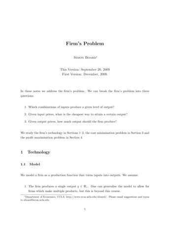
Eco11, Fall 2009Simon BoardFigure 1: Isoquant. This figure shows two isoquants. Each curve depicts the bundles that yieldconstant output.A firm has a collection of isoquants, each one corresponding to a different level of output. Byvarying this level, we can trace out the agent’s entire production possibilities.To illustrate, suppose a firm has production technology1/3 1/3f (z1 , z2 ) z1 z21/3 1/3Then the isoquant satisfies the equation z1 z2z2 k. Rearranging, we can solve for z2 , yieldingk3z1(1.1)which is the equation of a hyperbola. This function is plotted in figure 1.1.3Marginal Rate of Technical SubstitutionThe slope of the isoquant measures the rate at which the agent is willing to substitute one goodfor another. This slope is called the marginal rate of technical substitution or MRTS.Mathematically,dz2 M RT S dz1 f (z1 ,z2 ) const.3(1.2)

Eco11, Fall 2009Simon BoardWe can rephrase this definition in words: the MRTS equals the number of z2 the firm canexchange for one unit of z1 in order to keep output constant.The MRTS can be related to the firm’s production function. Let us consider the effect of asmall change in the firm’s inputs. Totally differentiating the production function f (z1 , z2 ) weobtaindq f (z1 , z2 ) f (z1 , z2 )dz1 dz2 z1 z2(1.3)Equation (1.3) says that the firm’s output increases by the marginal product of input 1 timesthe increase in input 1 plus the marginal product of input 2 times the increase in input 2. Alongan isoquant dq 0, so equation (1.3) becomes f (z1 , z2 ) f (z1 , z2 )dz1 dz2 0 z1 z2Rearranging, dz2 f (z1 , z2 )/ z1 dz1 u(z1 , z2 )/ z2Equation (1.2) therefore implies thatM RT S M P1M P2(1.4)The intuition behind equation (1.4) is as follows. Using the definition of MRTS, one unit of z1is worth MRTS units of z2 . That is, M P1 M RT S M P2 . Rewriting this equation we obtain(1.4).1.4Properties of TechnologyIn this section we present three properties of production functions that will prove useful.1. Monotonicity. The production function is monotone if for any two input bundles z (z1 , z2 )and z 0 (z10 , z20 ),zi zi0 for each i ozi zi0 for some iimplies f (z1 , z2 ) f (z10 , z20 ).In words: the production function is monotone if more of any input strictly increases thefirm’s output. Monotonicity implies that isoquants are thin and downwards sloping (see thePreferences Notes). As a result, it implies that MRTS is positive.4

Eco11, Fall 2009Simon Board2. Quasi–concavity. Let z (z1 , z2 ) and z 0 (z10 , z20 ). The production function is quasi–concaveif whenever f (z) f (z 0 ) thenf (tz (1 t)z 0 ) f (z 0 )for all t [0, 1](1.5)Suppose z and z 0 are two input bundles that produce the same output, f (z) f (z 0 ). Then(1.5) says a mixture of these bundles produces even more output. That is, mixtures of inputsare better than extremes.Under the assumption of monotonicity, quasi–concavity says that isoquants are convex. Thismeans that the MRTS decreasing in z1 along the isoquant. Formally, an isoquant defines animplicit relationship between z1 and z2 ,f (z1 , z2 (z1 )) kConvexity then implies that M RT S(z1 , z2 (z1 )) is decreasing in z1 . This is illustrated in Preferences Notes.3. Returns to Scale. A production function has decreasing returns to scale iff (tz1 , tz2 ) tf (z1 , z2 )for t 1(1.6)so that doubling the inputs less that doubles the output. A production function has constantreturns to scale iff (tz1 , tz2 ) tf (z1 , z2 )for t 1so that doubling the inputs also doubles output. Finally, a production function has increasingreturns to scale iff (tz1 , tz2 ) tf (z1 , z2 )for t 1so that doubling the inputs more than doubles the output.We will sometimes use the assumption that the production function f (z1 , z2 ) is concave. Thatis, for z (z1 , z2 ) and z 0 (z10 , z20 ),f (tz (1 t)z 0 ) tf (z) (1 t)f (z 0 )for t [0, 1](1.7)Concavity implies that the production function is quasi–concave (1.5) and hence that isoquantsare convex. This follows immediately from definitions: if f (z) f (z 0 ) then concavity (1.7)5

Eco11, Fall 2009Simon Boardimpliesf (tz (1 t)z 0 ) tf (z) (1 t)f (z 0 ) f (z 0 )so the production function is quasi–concave. In addition, concavity implies decreasing returnsto scale. Applying the definition of concavity (1.7) to the points z sz 00 and z 0 0 for s 1,and letting t 1/s, we obtainµfµ¶ ¶µ¶1111(sz) 1 0 f (sz) 1 f (0)ssssUsing f (0) 0 and simplifying, we obtain (1.7)2Examples of Production FunctionsHere we present some examples of production functions. Many details are omitted since this arepetition of the examples of utility functions.2.1Cobb DouglasA Cobb–Douglas production function is given byf (z1 , z2 ) z1α z2βfor α 0 and β 0Typical isoquants are shown in figure 1. The marginal products are given byM P1 αz1α 1 z2βM P2 βz1α z2β 1The marginal rate of technical substitution isM RT S M P1αz2 M P2βz1The returns to scale are easy to evaluate.f (tz1 , tz2 ) (tz1 )α (tz2 )β t tα β z1α z2β tα β f (z1 , z2 )6

Eco11, Fall 2009Simon BoardFigure 2: Isoquants for Leontief Technology. The isoquants are L–shaped, with the kink along theline αz1 βz2 .Hence there are decreasing returns if α β 1, constant returns if α β 1 and increasingreturns if α β 1.Exercise: Assume α β 1. Show that f (z1 , z2 ) is concave.12.2Perfect Complements (Leontief )A Leontief production function is given byf (z1 , z2 ) min{αz1 , βz2 }The isoquants are shown in figure 2. These are L–shaped with a kink along the line αz1 βz2 .This production function exhibits constant returns to scale.2.3Perfect SubstitutesWith perfect substitutes, the production function is given byf (z1 , z2 ) αz1 βz21For the definition of concavity with two variables, see the p. 5–6 of the math notes.7

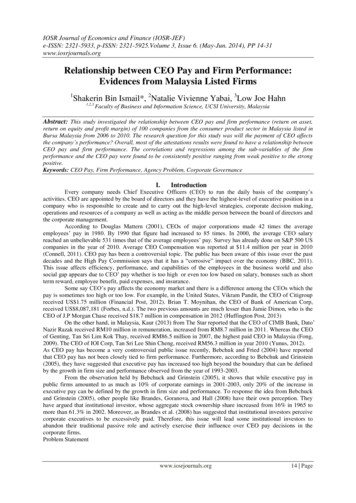
Eco11, Fall 2009Simon BoardFigure 3: Isoquants for Perfect Substitutes. The isoquants are straight line with slope α/β.The isoquants are shown in figure 3. These are straight lines with slope α/β. This productionfunction exhibits constant returns to scale.3Cost Minimisation Problem (CMP)We make several assumptions:1. There are N inputs. For much of the analysis we assume N 2 but nothing depends onthis.2. The agent takes input prices as exogenous. We assume these prices are linear and strictlypositive and denote them by {r1 , . . . , rN }.3. The firm has production technology f (z1 , z2 ). We normally assume that the productionfunction is differentiable, which ensures that any optimal solution satisfies the Kuhn–Tucker conditions. If the production function is quasi–concave and M Pi (z1 , z2 ) 0 forall (z1 , z2 ), then any solutions to the Kuhn–Tucker conditions are optimal. See Section4.1 of the UMP notes for more details.8

Eco11, Fall 20093.1Simon BoardCost Minimisation ProblemThe cost minimisation problem isminNXz1 ,.,zNri zisubject tof (z1 , . . . , zN ) q(3.1)i 1zi 0 for all iThe idea is that the firm is trying to find the cheapest way to attain a certain output, q. Thesolution to this problem yields the firm’s input demands which are denoted byzi (r1 , . . . , rN , q)The money the firm must spend in order to attain its target output is its cost. The costfunction is thereforec(r1 , . . . , rN , q) minz1 ,.,zNNXri zisubject tof (z1 , . . . , zN ) qi 1zi 0 for all iEquivalently, the cost function equals the amount the firm spends on her optimal inputs,c(r1 , . . . , rN , q) NXri zi (r1 , . . . , rN , q)(3.2)i 1Note this problem is formally identical to the agent’s expenditure minimisation problem. Thecost function is therefore equivalent to the agent’s expenditure function.Given a cost function, the average cost is,AC(r1 , r2 , q) c(r1 , r2 , q)qThe marginal cost equals the cost of each additional unit,M C(r1 , r2 , q) 9dc(r1 , r2 , q)dq

Eco11, Fall 2009Simon BoardFigure 4: Constraint Set. This figure shows the set of inputs that deliver the target output, q.3.2Graphical SolutionThe firm wishes to find the cheapest way to attain a certain output.First, we need to understand the constraint set. The firm can choose any bundle of inputswhere (a) the firm attains her target output, f (z1 , z2 ) q; and (b) the quantities are positive,z1 0 and z2 0. If the firm’s production function is monotone, then the bundles that meetthese conditions are the ones that lie above the isoquant with output q. See figure 4.Second, we need to understand the objective. The firm wishes to pick the bundle in theconstraint set that minimises her cost. Define an isocost curve by the bundles of z1 and z2 thatdeliver constant cost:{(z1 , z2 ) : r1 z1 r2 z2 const.}These isocost curves are just like budget curves and so have slope r1 /r2 . See figure 5.Ignoring boundary problems and kinks, the solution to the CMP has the feature that the isocostcurve is tangent to the target isoquant. As a result, their slopes are identical. The tangencycondition can thus be written asM RT S This is illustrated in figure 6.10r1r2(3.3)

Eco11, Fall 2009Simon BoardFigure 5: Isocost. The isocost function shows the set of inputs which cost the same amount of money.Figure 6: Tangency. This figure shows that, at the optimal input combination, the isocost curve istangent to the isoquant.11