WIXLIB

Energies 2020, 13, 48003 of 33in the walls) and on the design of QUB experiment (heating power and duration). Development andvalidation of reliable procedures, with generalized applicability to in‐use buildings and including asunny and warm climate and capable of dealing with the dynamic features of these generalizedconditions, are also necessary to achieve the readiness required for deployment in this context.Uncertain accuracy, high cost and intrusiveness limit the implementation of some experimentalmethods. Additionally, the increasing availability of smart technologies and on‐board monitoringsystems offers a huge amount of data that could be used for the assessment of building energyperformance of in‐use buildings. The development and validation of reliable procedures togetherwith the access to smart technologies and on‐board monitoring systems could facilitate theintroduction of performance assessment procedures in normative and commercial applications.Dynamic issues are relevant to the energy performance of walls and whole buildings [25,26].Dynamic data‐based modelling techniques are promising to carry out the energy performanceassessment of in‐use buildings overcoming some problems that arise when some average and linearregression methods are applied. Wide activity has been developed in this area [3,27], with a broaddevelopment on techniques for the identification of the parameters characterizing the thermalperformance of building components, from dynamic tests in outdoor test cells, usually obtained fromlinear and time‐invariant models [28]. The extension and generalization of the current scope ofapplication of these techniques is not simple, but some researches are undertaking this challenge [29].This article deals with the application of RC dynamic models for assessing the in‐situ thermalperformance of walls (identifying the U value) and whole buildings (identifying the UA value andgA value). These models use an electrical analogy representing the thermal system to obtain therequired parameters. LORD software has been used as tool to identify the required parameters fromthe measured data series [30]. The potential to apply this approach to in‐use buildings has beendemonstrated by a previously published work [29]. This paper repots a further systematic analysisfocusing on the following aspects: the effect of the solar radiation on the heat flux through the opaquewalls versus the performance of the models including this effect. Although previous work [31]analyzed this issue applying another method and concluded that neglecting this effect is convenient,a deeper analysis is here reported. This work also studied the optimum number of nodes required torepresent the thermal systems, the assignment of inputs and outputs and the length of the test period.Additionally, several options modelling relevant effects using unmeasured variables were studied toevaluate the feasibility to reduce the cost and intrusiveness of the measurement devices required toobtain accurate results. The feasibility to model relevant effects using unmeasured variables has beendemonstrated.A building which is well‐known and simplified has been considered for this study. Data seriesrecorded under very different experimental conditions were used to analyze the robustness andvalidity of the results. The performance of the models for each of these different test conditions isdiscussed. The detailed information of the construction of the building which is available, includingaccurate geometrical parameters and thermal properties of its construction materials, strengthensand complements the criteria for validation. This issue together with the simplicity of the building,the oversizing of its test set up and length, and the richness of the weather conditions throughout thetest campaign, are relevant features to make this case study suitable to corroborate, complement, andextend some findings from previous works [31]. These analyses and comparisons give backgroundto support the criteria for selecting the best model among the considered candidates and theminimum set of variables required to guarantee an adequate accuracy of the analysis. The objectiveis to find the simplest and cheapest models giving enough accuracy. These requisites are crucialregarding deployment in commercial applications.The same benchmark data have been used as support to other research focusing on differentaspects and methodologies. Rouchier et al. [32] report the application of Sequential Monte Carlo(SMC) for the on‐line estimation of the heat loss coefficient (HLC) of a building. Chávez et al. [31]analyzed systematically different key aspects of a dynamic integrated method applied to assessingthe in‐situ thermal performance of walls and whole buildings and demonstrated the reliability of thatmethod.

Energies 2020, 13, 48004 of 33The analysis reported in this paper added to other published works [31] constitutes a collectionof methods systematically applied and validated by means of their application to the same test set upand high quality benchmark data. This material contributes as a strong basis and background to thedevelopment of procedures for the in‐situ performance assessment of the building fabric, using datarecorded by on‐board monitoring systems, from test campaigns conducted under a large variety ofweather and test conditions.The next sections are organized as follows: Section 2 briefly describes the simplified building,the boundary conditions and test set up used as a case study in this research work; Section 2 alsointroduces the methodology that has been applied as well as the steps followed for the analysis, firstof the opaque walls and afterwards of the whole building; Section 3 reports and discusses the results;and, finally, Section 4 synthesizes the main findings of the work.2. Materials and Methods2.1. Benchmark Set Up and DataA test box performing as a simplified building was used in this research work. It was built withinthe framework of IEA EBC Annex 58. The same building was used as benchmark and support forprevious research works in this context. This building and the experiment set up are briefly presentedhereafter. Further information is reported in reference [15].2.1.1. The Building (Test Box)The simplified building is a test box that consists of a cubic structure (Figure 1). Its exteriordimensions are 120 120 120 cm3, and the ceiling, floor and walls are all 12 cm thick. The south wallhas a wooden‐framed window 71 71 cm2 and a glazed area of 52 52 cm2. It is suspended over astructure that avoids contact with the ground. Due to its airtight construction, air leakage can beassumed as negligible.(a)(b)(c)Figure 1. Experiment set up. (a) Test box and measurement devices in its surroundings, (b) detail ofinstallation of indoor air temperature sensors protected by aluminum cylinders, (c) detail ofinstallation of shielded and ventilated outdoor air temperature sensors.The thermal transmittance (U in Wm 2K 1) and the solar‐energy transmittance (g, dimensionless)have been considered to characterize the opaque elements (ceiling, floor and walls) from one‐dimensional analysis. The overall thermal transmission coefficient (UA in WK 1) and the total solarheat gain factor (gA in m2), have been considered to characterize the whole building envelope fromthree‐dimensional analysis. The values of the characteristic parameters of the building theoreticallycalculated, together with the results obtained applying other method for the analysis were used ascomplement to the validation criteria (Table 1). The maximum deviations for the theoretical valueswere calculated as the standard deviation among all the average values for winter and summer dataseries due to variations of surface temperature and wind speed, which are minor deviations, as

Energies 2020, 13, 48005 of 33shown in Table 1. The g value is very low. According to [15], it is 0.0060 in average. Taking intoaccount this low value it could lead to an undetectable effect of the solar radiation on the interiorsurfaces of the opaque walls.Table 1. Theoretical values of the characteristic parameters and estimated ranges of deviations fromtheir constant values, and values obtained applying other analysis method [31].ParametersU Ceiling (W/m2K)U Back (W/m2K)U Right Wall (W/m2K)U Left Wall (W/m2K)UA Whole Box (W/K)gA Whole Box aximumDeviation0.003 (0.7%)0.003 (0.7%)0.003 (0.7%)0.003 (0.7%)0.03 (0.7%)0.00002 (0.01%)Value from DynamicIntegrated Method [31]0.50 (1.0%)0.45 (0.03%)0.45 (2.5%)0.45 (1.0%)4.08 (0.6%)0.160 (1.7%)2.1.2. Boundary ConditionsThe test campaign was carried out outdoors at the Plataforma Solar de Almeria (PSA), in thesouth east of Spain (37.1 N, 2.4 W). The area is rural, and the climate is typically hot and dry insummer and cold in winter; the air temperature presents large oscillations from day to night, withhigh levels solar radiation and clear sky.2.1.3. Conducted Experiments and Data SeriesSeveral experiments have been conducted under different test conditions to obtain different dataseries which are suitable to analyze different aspects of the modelling methods. The heating powerwas supplied by a 100 W incandescence lamp and the indoor air temperatures have been controlledin order to set the different test conditions. The experiment set up includes a comprehensive set ofmeasurement devices [15]. The following subset of variables has been used for the analysis describedin the next sections: Indoor air temperature, Ti, as the average of the two measurements of this variable Ti down andTi up, shown in Figure 1b.Outdoor air temperature, Te, as the average of the two measurements of this variable Te middle andTe down, shown in Figure 1c.Measured heat flux through ceiling, floor and all the opaque walls: φceiling, φfloor, φback, φleft andφright.Measured heating power, Pheating.Measured global vertical solar radiation facing south, Gv.The experiments have been designed aiming to produce several data series containing theinformation required to apply system identification techniques. The phenomena to be characterizedmust be evident and strong enough for the application of these techniques. In this context, aphenomenon is strong enough when the amplitude of its driving variable is significantly higher thanthe uncertainty in its measurement. If a driving variable does not fit this requisite, signal to noise ispoor, leading to inaccurate parameter estimates. Accordingly: To identify the heat transfer coefficient, the test set‐up must guarantee strong enough heat lossthrough the building envelope maximizing the indoor to outdoor air temperature difference,which is the driving variable for this effect.To identify the overall gA‐value, the solar gains must be strong enough. This is achieved whenthe test period includes enough sunny days with high levels of solar radiation, which is thecorresponding driving variable.To identify dynamic models, the system must be excited by dynamic input signals containing awide range of frequencies and including the characteristic time constants of the system. The

Energies 2020, 13, 48006 of 33variables involved in the energy balance equations of outdoor tests have a dynamic character,but identification is facilitated by the application of certain power sequences such as the ROLBS[33] etc.The following issues regarding the experiment set up are also relevant to the identifiability andaccuracy of the parameter estimates: Heating Power: heating the indoor air is necessary to maximize the indoor to outdoor airtemperature difference. Free running tests usually lead to poor signal to noise ratios in themeasurements of temperature difference and cause problems with identifiability. Additionally,the heating power must be strong enough because it is a relevant variable to the energy balanceequation that must be used for the analysis.Homogeneity of the indoor air temperature: the solar radiation and the heating systems areheating sources that can produce some inhomogeneity to the indoor air temperature whichcontribute to the uncertainty of the parameter estimates. A mini fan has been used to improvethe air temperature homogeneity. A device with very small ventilation power has been chosento avoid perturbations in the interior convection coefficients.Sampling frequency: the sampling theorem must be fulfilled in the raw data as well as in anyresampling applied in the pre‐processing phase. The sampling frequency must be at least twicethe frequency of the variable which is being measured.According to all these issues three data series corresponding to different periods have beenconsidered. One‐minute sampling interval has been set. This sampling interval guarantees that theraw data fulfil the sampling theorem. The main differences among the three periods concerns to theheating power and indoor temperature settings: Series 16: 6 December 2013 to 17 December 2013 (12 days). This series includes one ROLBS powersequence and was mainly designed to optimize the test conditions to the application of thesystem identifications techniques.Series 17: 18 December 2013 to 26 December 2013 (9 days). Aiming to reproduce as possible acoheating test, but setting the indoor air temperature set point to 35 C. This test sequence wasdesigned in order to have a reference analysis according as much as possible to the traditionalcoheating test, and also to explore the application of steady‐state approaches and also to analyzethe capability to apply the system identification techniques to this type of tests. This series is alsouseful to analyze causality issues and different variables as the input signal. It must be observedthat this test is not identical to the coheating test described in the literature [17]. It is a bitmodified taking into account the given boundary conditions: in winter the indoor airtemperature cannot be maintained at a constant 25 C because the low position of the sunproduces a strong global solar radiation incident on the window (Figure 2e). Consequently, theindoor air temperature shows some dynamic behavior with overheating intervals (Figure 2d)even raising the set point to 35 C.Series 18: 27 December 2013 to 7 January 2014 (12 days): also aiming to reproduce as possible aCoheating test, but in this case setting the indoor air temperature set point to 21 C, intending toemulate the comfort zone in an in‐use building. These more realistic conditions are set in orderto explore the possibilities to apply these identification techniques to in‐use buildings using datarecorded by its on‐board monitoring systems. These test conditions are also interesting toanalyze causality issues and different variables as output signals. In this case, the low level ofthe indoor to outdoor air temperature difference increases the difficulty to identify the UA value.Additionally, the contribution of the solar radiation to the space heating makes it impossible tomaintain a constant indoor air temperature. This effect, clearly seen from the observation ofFigure 2e,f, is stressing the need to apply dynamic techniques for the analysis.Finally, the consecutive records available in these data series have been merged in one data seriesand then this full data series has been split in three series with identical length. The analysis has beendone using the resulting four data series, named as:

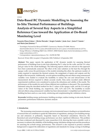
Energies 2020, 13, 4800200Temperature ( 342344346348350352Time (Days)352Time (Days)Te middleP heatingTe down(a)Ti downTi up(b)200Temperature ( 359361Time (Days)361Time (Days)Te middleP heatingTe down(c)Ti downTi up(d)401200Temperature ( C) Heating Power (W) Haeting Power (W) Series a: 6 December 2013 to 16 December 2013 (11 days). The test conditions in this series aredominated by the test conditions in series 16, with a ROLBS power sequence.Series b: 17 December 2013 to 27 December 2013 (11 days). The test conditions in this series aredominated by the test conditions in series 17, mainly with 35 C set point for the indoor airtemperature which is mainly constant.Series c: 28 December 2013 to 7 January 2014 (11 days): The test conditions in this series aredominated by the test conditions in series 18, mainly with 21 C set point for the indoor airtemperature trying to maintain a constant indoor air temperature which actually has a dynamicbehavior.Series d: 6 December 2013 to 7 January 2014 (33 days), which is the combination of series 16, 17and 18, therefore including a rich diversity of test conditions.Radiation (W/m2) 7 of 69371373Time (Days)373Time (Days)GvGh(e)Te middleTe downTi downTi up(f)Figure 2. Data overview where Pheating is the heating Power; Gv and Gh are the vertical and thehorizontal global solar radiation, Ti down and Ti up are the two measurements of the indoor airtemperature, Te middle and Te down are the two measurements of the outdoor air temperatures. (a)Heating power. Series 16, (b) indoor and outdoor air temperatures. Series 16, (c) heating power. Series17, (d) indoor and outdoor air temperatures. Series 17, (e) vertical and horizontal global solarradiation. Series 18, (f) indoor and outdoor air temperatures. Series 18.

Energies 2020, 13, 48008 of 332.2. Data Analysis and Modelling MethodologyThe subsequent subsections describe the following issues of the methodology that has beenapplied: First, the dynamic RC modelling approach is briefly presented (in Section 2.2.1). The criteriato assess performance of the models and the validity of the results are presented (in Section 2.2.2).Then the application of this methodology to the ceiling, floor, opaque walls (in Section 2.2.3) and thewhole building (in Section 2.2.4) is described. Afterwards, some models including modelling of someeffects driven by unmeasured variables are considered (in Section 2.2.5).Several candidate models have been considered. All these candidate models have beenconstructed translating the physical features of the considered thermal systems into RC modelstructures. Simplifications, in which validity was demonstrated in previous work [31], were takeninto account to construct these RC models. Accordingly, the starting points of this work are the resultsand conclusions reported in [31]. This work explores the capabilities of RC models to improve theresults of that work analyzing the following aspects: Further analysis of the influence of the solar radiation that is transmitted through the opaquewalls versus the performance of the models including this effect. The work reported in [31]concluded that including the solar radiation in the models of the opaque walls does not improvethe accuracy of the U value estimates. However, a model including a y‐intercept was identifiedas the best model among the considered candidate models. The y‐intercept was interpreted as arepresentation of the sum of the effects that were not included explicitly in the model. This issueinduced us to carry out further analysis reconsidering the effect of the solar radiation applyingthe RC approach described in this paper.Other effects such as dependencies on wind speed, surface and fabric temperatures have beendisregarded taking into account the conclusions of the work reported in [31].Several options modelling relevant effects using unmeasured variables in order to evaluate thefeasibility to reduce the cost and intrusiveness of the measurement devices required us to obtainaccurate results. These options were not considered in [31]. However other works havedemonstrated the usefulness of modelling several effects which are driven by unmeasuredvariables [34,35].Additionally, the following issues of the RC modelling approach have been investigated alongthe application of this method to the particular case study considered in this work: Reduction of the test period regarding the test period required us to obtain accurate resultsapplying the dynamic integrated method applied in [31].The optimum number of nodes required to represent the thermal systems.The assignment of inputs and outputs.The performance of the models using data recorded under different test conditions.2.2.1. RC ModelsRC models are used for obtaining the U value of the opaque walls and the UA value and gAvalue of the whole building. These models use an electrical analogy representing the thermal systemto obtain the required parameters. The software tool LORD [30] has been used to identify theparameters of these models. Physical criteria have been combined with this modelling approach toobtain these coefficients and also to validate the results. This applied approach is based on energybalances, constructed from the main heat transfer contributions that are identified and modelled.First, the U values of the opaque walls, ceiling and floor were obtained by a one‐dimensionalanalysis based on direct measurement of heat flux through the interior surfaces. The main focus ofthis analysis was determining the optimum number of nodes to represent the opaque walls.Afterwards, a three‐dimensional analysis based on the energy balance on the air volume confined bythe building envelope, was applied to estimate the overall UA and gA values of the whole buildingenvelope. The data series a, b, c and d recorded under different test conditions as well as the results

Energies 2020, 13, 48009 of 33obtained in previous work, applying a different method [31] and also the target design values, wereused to analyze the robustness of the results.2.2.2. Assessment of the Validity of the ResultsThe performance of the candidate modes to give accurate estimates of the required ch

In‐Situ Thermal Performance of Buildings. Analysis of Several Key Aspects in a Simplified Reference Case toward the Application at On‐Board Monitoring Level Yessenia Olazo‐Gómez 1, Héctor Herrada 2, Sergio Castaño 2, Jesús Arce 1, Jesús P. Xamán 1 and María José Jiménez 2,*