Transcription
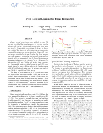
Deep Residual Learning for Image RecognitionKaiming HeXiangyu ZhangShaoqing RenMicrosoft ResearchJian Sun{kahe, v-xiangz, v-shren, jiansun}@microsoft.com1. IntroductionDeep convolutional neural networks [22, 21] have ledto a series of breakthroughs for image classification [21,49, 39]. Deep networks naturally integrate low/mid/highlevel features [49] and classifiers in an end-to-end multilayer fashion, and the “levels” of features can be enrichedby the number of stacked layers (depth). Recent evidence[40, 43] reveals that network depth is of crucial importance,and the leading results [40, 43, 12, 16] on the challengingImageNet dataset [35] all exploit “very deep” [40] models,with a depth of sixteen [40] to thirty [16]. Many other nontrivial visual recognition tasks [7, 11, 6, 32, 27] have also1 1056-layertest error (%)Deeper neural networks are more difficult to train. Wepresent a residual learning framework to ease the trainingof networks that are substantially deeper than those usedpreviously. We explicitly reformulate the layers as learning residual functions with reference to the layer inputs, instead of learning unreferenced functions. We provide comprehensive empirical evidence showing that these residualnetworks are easier to optimize, and can gain accuracy fromconsiderably increased depth. On the ImageNet dataset weevaluate residual nets with a depth of up to 152 layers—8 deeper than VGG nets [40] but still having lower complexity. An ensemble of these residual nets achieves 3.57% erroron the ImageNet test set. This result won the 1st place on theILSVRC 2015 classification task. We also present analysison CIFAR-10 with 100 and 1000 layers.The depth of representations is of central importancefor many visual recognition tasks. Solely due to our extremely deep representations, we obtain a 28% relative improvement on the COCO object detection dataset. Deepresidual nets are foundations of our submissions to ILSVRC& COCO 2015 competitions1 , where we also won the 1stplaces on the tasks of ImageNet detection, ImageNet localization, COCO detection, and COCO segmentation.20training error (%)Abstract56-layer20-layer1020-layer001234iter. (1e4)5600123456iter. (1e4)Figure 1. Training error (left) and test error (right) on CIFAR-10with 20-layer and 56-layer “plain” networks. The deeper networkhas higher training error, and thus test error. Similar phenomenaon ImageNet is presented in Fig. 4.greatly benefited from very deep models.Driven by the significance of depth, a question arises: Islearning better networks as easy as stacking more layers?An obstacle to answering this question was the notoriousproblem of vanishing/exploding gradients [14, 1, 8], whichhamper convergence from the beginning. This problem,however, has been largely addressed by normalized initialization [23, 8, 36, 12] and intermediate normalization layers[16], which enable networks with tens of layers to start converging for stochastic gradient descent (SGD) with backpropagation [22].When deeper networks are able to start converging, adegradation problem has been exposed: with the networkdepth increasing, accuracy gets saturated (which might beunsurprising) and then degrades rapidly. Unexpectedly,such degradation is not caused by overfitting, and addingmore layers to a suitably deep model leads to higher training error, as reported in [10, 41] and thoroughly verified byour experiments. Fig. 1 shows a typical example.The degradation (of training accuracy) indicates that notall systems are similarly easy to optimize. Let us consider ashallower architecture and its deeper counterpart that addsmore layers onto it. There exists a solution by constructionto the deeper model: the added layers are identity mapping,and the other layers are copied from the learned shallowermodel. The existence of this constructed solution indicatesthat a deeper model should produce no higher training errorthan its shallower counterpart. But experiments show thatour current solvers on hand are unable to find solutions that1770
xweight layerF(x)reluxweight layerF(x) xidentityreluFigure 2. Residual learning: a building block.are comparably good or better than the constructed solution(or unable to do so in feasible time).In this paper, we address the degradation problem byintroducing a deep residual learning framework. Instead of hoping each few stacked layers directly fit adesired underlying mapping, we explicitly let these layers fit a residual mapping. Formally, denoting the desiredunderlying mapping as H(x), we let the stacked nonlinearlayers fit another mapping of F(x) : H(x) x. The original mapping is recast into F(x) x. We hypothesize that itis easier to optimize the residual mapping than to optimizethe original, unreferenced mapping. To the extreme, if anidentity mapping were optimal, it would be easier to pushthe residual to zero than to fit an identity mapping by a stackof nonlinear layers.The formulation of F(x) x can be realized by feedforward neural networks with “shortcut connections” (Fig. 2).Shortcut connections [2, 33, 48] are those skipping one ormore layers. In our case, the shortcut connections simplyperform identity mapping, and their outputs are added tothe outputs of the stacked layers (Fig. 2). Identity shortcut connections add neither extra parameter nor computational complexity. The entire network can still be trainedend-to-end by SGD with backpropagation, and can be easily implemented using common libraries (e.g., Caffe [19])without modifying the solvers.We present comprehensive experiments on ImageNet[35] to show the degradation problem and evaluate ourmethod. We show that: 1) Our extremely deep residual netsare easy to optimize, but the counterpart “plain” nets (thatsimply stack layers) exhibit higher training error when thedepth increases; 2) Our deep residual nets can easily enjoyaccuracy gains from greatly increased depth, producing results substantially better than previous networks.Similar phenomena are also shown on the CIFAR-10 set[20], suggesting that the optimization difficulties and theeffects of our method are not just akin to a particular dataset.We present successfully trained models on this dataset withover 100 layers, and explore models with over 1000 layers.On the ImageNet classification dataset [35], we obtainexcellent results by extremely deep residual nets. Our 152layer residual net is the deepest network ever presented onImageNet, while still having lower complexity than VGGnets [40]. Our ensemble has 3.57% top-5 error on theImageNet test set, and won the 1st place in the ILSVRC2015 classification competition. The extremely deep representations also have excellent generalization performanceon other recognition tasks, and lead us to further win the1st places on: ImageNet detection, ImageNet localization,COCO detection, and COCO segmentation in ILSVRC &COCO 2015 competitions. This strong evidence shows thatthe residual learning principle is generic, and we expect thatit is applicable in other vision and non-vision problems.2. Related WorkResidual Representations. In image recognition, VLAD[18] is a representation that encodes by the residual vectorswith respect to a dictionary, and Fisher Vector [30] can beformulated as a probabilistic version [18] of VLAD. Bothof them are powerful shallow representations for image retrieval and classification [4, 47]. For vector quantization,encoding residual vectors [17] is shown to be more effective than encoding original vectors.In low-level vision and computer graphics, for solving Partial Differential Equations (PDEs), the widely usedMultigrid method [3] reformulates the system as subproblems at multiple scales, where each subproblem is responsible for the residual solution between a coarser and a finerscale. An alternative to Multigrid is hierarchical basis preconditioning [44, 45], which relies on variables that represent residual vectors between two scales. It has been shown[3, 44, 45] that these solvers converge much faster than standard solvers that are unaware of the residual nature of thesolutions. These methods suggest that a good reformulationor preconditioning can simplify the optimization.Shortcut Connections. Practices and theories that lead toshortcut connections [2, 33, 48] have been studied for a longtime. An early practice of training multi-layer perceptrons(MLPs) is to add a linear layer connected from the networkinput to the output [33, 48]. In [43, 24], a few intermediate layers are directly connected to auxiliary classifiersfor addressing vanishing/exploding gradients. The papersof [38, 37, 31, 46] propose methods for centering layer responses, gradients, and propagated errors, implemented byshortcut connections. In [43], an “inception” layer is composed of a shortcut branch and a few deeper branches.Concurrent with our work, “highway networks” [41, 42]present shortcut connections with gating functions [15].These gates are data-dependent and have parameters, incontrast to our identity shortcuts that are parameter-free.When a gated shortcut is “closed” (approaching zero), thelayers in highway networks represent non-residual functions. On the contrary, our formulation always learnsresidual functions; our identity shortcuts are never closed,and all information is always passed through, with additional residual functions to be learned. In addition, high2771
way networks have not demonstrated accuracy gains withextremely increased depth (e.g., over 100 layers).3. Deep Residual Learning3.1. Residual LearningLet us consider H(x) as an underlying mapping to befit by a few stacked layers (not necessarily the entire net),with x denoting the inputs to the first of these layers. If onehypothesizes that multiple nonlinear layers can asymptotically approximate complicated functions2 , then it is equivalent to hypothesize that they can asymptotically approximate the residual functions, i.e., H(x) x (assuming thatthe input and output are of the same dimensions). Sorather than expect stacked layers to approximate H(x), weexplicitly let these layers approximate a residual functionF(x) : H(x) x. The original function thus becomesF(x) x. Although both forms should be able to asymptotically approximate the desired functions (as hypothesized),the ease of learning might be different.This reformulation is motivated by the counterintuitivephenomena about the degradation problem (Fig. 1, left). Aswe discussed in the introduction, if the added layers canbe constructed as identity mappings, a deeper model shouldhave training error no greater than its shallower counterpart. The degradation problem suggests that the solversmight have difficulties in approximating identity mappingsby multiple nonlinear layers. With the residual learning reformulation, if identity mappings are optimal, the solversmay simply drive the weights of the multiple nonlinear layers toward zero to approach identity mappings.In real cases, it is unlikely that identity mappings are optimal, but our reformulation may help to precondition theproblem. If the optimal function is closer to an identitymapping than to a zero mapping, it should be easier for thesolver to find the perturbations with reference to an identitymapping, than to learn the function as a new one. We showby experiments (Fig. 7) that the learned residual functions ingeneral have small responses, suggesting that identity mappings provide reasonable preconditioning.3.2. Identity Mapping by ShortcutsWe adopt residual learning to every few stacked layers.A building block is shown in Fig. 2. Formally, in this paperwe consider a building block defined as:y F(x, {Wi }) x.(1)Here x and y are the input and output vectors of the layers considered. The function F(x, {Wi }) represents theresidual mapping to be learned. For the example in Fig. 2that has two layers, F W2 σ(W1 x) in which σ denotes2 Thishypothesis, however, is still an open question. See [28].ReLU [29] and the biases are omitted for simplifying notations. The operation F x is performed by a shortcutconnection and element-wise addition. We adopt the second nonlinearity after the addition (i.e., σ(y), see Fig. 2).The shortcut connections in Eqn.(1) introduce neither extra parameter nor computation complexity. This is not onlyattractive in practice but also important in our comparisonsbetween plain and residual networks. We can fairly compare plain/residual networks that simultaneously have thesame number of parameters, depth, width, and computational cost (except for the negligible element-wise addition).The dimensions of x and F must be equal in Eqn.(1).If this is not the case (e.g., when changing the input/outputchannels), we can perform a linear projection Ws by theshortcut connections to match the dimensions:y F(x, {Wi }) Ws x.(2)We can also use a square matrix Ws in Eqn.(1). But we willshow by experiments that the identity mapping is sufficientfor addressing the degradation problem and is economical,and thus Ws is only used when matching dimensions.The form of the residual function F is flexible. Experiments in this paper involve a function F that has two orthree layers (Fig. 5), while more layers are possible. But ifF has only a single layer, Eqn.(1) is similar to a linear layer:y W1 x x, for which we have not observed advantages.We also note that although the above notations are aboutfully-connected layers for simplicity, they are applicable toconvolutional layers. The function F(x, {Wi }) can represent multiple convolutional layers. The element-wise addition is performed on two feature maps, channel by channel.3.3. Network ArchitecturesWe have tested various plain/residual nets, and have observed consistent phenomena. To provide instances for discussion, we describe two models for ImageNet as follows.Plain Network. Our plain baselines (Fig. 3, middle) aremainly inspired by the philosophy of VGG nets [40] (Fig. 3,left). Th
Microsoft Research {kahe, v-xiangz, v-shren, jiansun}@microsoft.com Abstract Deeper neural networks are more difficult to train. We present a residual learning framework to ease the training of networks that are substantially deeper than those used previously. We explicitly reformulate the layers as learn-