WIXLIB

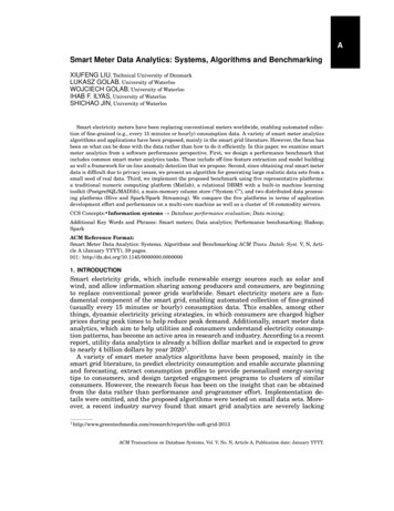
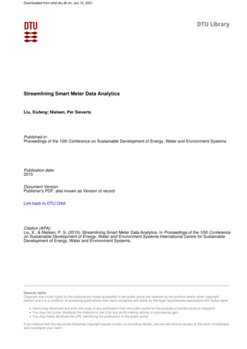
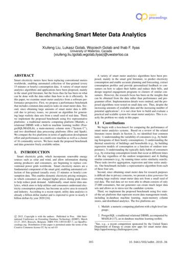
3.Consump(on)(kWh))We also note that the TCP benchmarks include the ability to generate very large synthetic databases, and there has been some research on synthetic database generation (see, e.g., [11]), but we arenot aware of any previous work on generating realistic smart meterdata.THE BENCHMARKIn this section, we propose a performance benchmark for smartmeter analytics. The primary goal of the benchmark is to measurethe running time of a set of tasks that will be defined shortly. Theinput consists of n time series, each corresponding to one electricity consumer, in one or more text files. We assume that eachtime series contains hourly electricity consumption measurements(in kilowatt-hours, kWh) for a year, i.e., 365 24 8760 datapoints. For each consumption time series, we require an accompanying external temperature time series, also with hourly measurements.For each task, we measure the running time on the input data set,both with a cold start (working directly from the raw files) and awarm start (working with data loaded into physical memory). Inthis version of the benchmark, we do not consider the cost of updates, e.g., adding a day’s worth of new points to each time series.However, adding updates to the benchmark is an important direction for future work as read-optimized data structures that help improve running time may be expensive to update.Utility companies may have access to additional data about theircustomers, e.g., location, square footage of the home or family size.However, this information is usually not available to third-partyapplications. Thus, the input to our benchmark is limited to thesmart meter time series and publicly-available weather data.We now discuss the four analysis tasks included in the ))))35)External)temperature)(degrees)C))Figure 1: Example of the 3-line regression model.value and then computes the two sets of regression lines. In the finalstep, the algorithm ensures that the three lines are not discontinuousand therefore it may need to adjust the lines slightly.As shown in Figure 1, the 3-line algorithm extracts useful information for customer feedback. For instance, the slopes (gradients)of the left and right 90th percentile lines correspond to the heating and cooling sensitivity, respectively. A high cooling gradientmight indicate an inefficient air conditioning system or a low airconditioning set point. Additionally, the height at the lowest pointon the 10th percentile lines indicates base load, which is the electricity consumption of appliances and devices that are always onregardless of the temperature (e.g., a refrigerator, a dehumidifier,or a home security system).Consumption Histograms3.3The first task is to understand the variability of each consumer.To do this, we compute the distribution of hourly consumption foreach consumer via a histogram. The x-axis in the histogram denotes various hourly consumption ranges and the y-axis is the frequency, i.e., the number of hours in the year whose electricity consumption falls in the given range. For concreteness, in the proposedbenchmark we specify the histograms to be equi-width (rather thanequi-depth) and we always use ten buckets.3.2cooling)gradient)hea(ng)gradient)Daily ProfilesThe third task is to extract daily consumption trends that occurregardless of the outdoor temperature. For this, we use the periodicautoregression (PAR) algorithm for time series data from [8, 13].The idea behind this algorithm is illustrated in Figure 2. At the top,we show a fragment of the hourly consumption time series for someconsumer over a period of several days. We are only given the totalhourly consumption, but the goal of the algorithm is to determine,for each hour, how much load is temperature-independent and howmuch additional load is due to temperature (i.e., heating or cooling). Once this is determined, the algorithm computes the averagetemperature-independent consumption at each hour of the day, illustrated at the bottom of Figure 2. Thus, for each consumer, theoutput consists of a vector of 24 numbers, denoting the expectedconsumption at different hours of the day due solely to the occupants’ daily habits and not affected by temperature.For each consumer and each hour of the day, the PAR algorithmfits an auto-regressive model, which assumes that the electricityconsumption at that hour of the day is a linear combination of theconsumption at the same hour over the previous p days (we use p 3, as in [8]) and the outdoor temperature. Thus, it groups the inputdata set by consumer and by hour, and computes the coefficients ofthe auto-regressive model for each group.Thermal SensitivityThe second task is to understand the effect of outdoor temperature on the electricity consumption of each household. Thesimplest approach is to fit a least-squares regression line to theconsumption-temperature scatter plot. However, in climates with acold winter and warm summer, electricity consumption rises whenthe temperature drops in the winter (due to heating) and also riseswhen the temperature rises in the summer (due to air conditioning).Thus, a piecewise linear regression model is more appropriate.We selected the recently-proposed algorithm from [10] for thebenchmark, to which we refer as the 3-line algorithm. Consider aconsumption-temperature scatter plot for a single consumer shownin Figure 1 (the actual points are not shown, but a point on this plotwould correspond to a particular hourly consumption value and theoutdoor temperature at that hour). The upper three lines correspondto the piecewise regression lines computed only for the points inthe 90th percentile for each temperature value and the lower threelines are computed from the points in the 10th percentile for eachtemperature value. Thus, for each time series, the algorithm startsby computing the 10th and 90th percentiles for each temperature3.4Similarity SearchThe final task is to find groups of similar consumers. Customersegmentation is important to utilities so they can determine howmany distinct groups of customers there are and design targetedenergy-saving campaigns for each group. Rather than choosing387

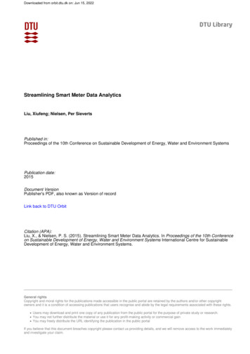
Consump,on%(kWh)%benchmark with increasing values of n. Since it is difficult to obtain large amounts of smart meter data due to privacy issues, andsince using randomly-generated time series may not give accurateresults, we propose a data generator for realistic smart meter data.The intuition behind the data generator is as follows. Since electricity consumption depends on external temperature and daily activity, we start with a small seed of real data and we generate thedaily activity profiles (recall Figure 2) and temperature regressionlines (recall Figure 1) for each consumer therein. To generate anew time series, we take the daily activity pattern from a randomlyselected consumer in the real data set, the temperature dependencyfrom another randomly-selected consumer, and we add some whitenoise. Thus, we first disaggregate the consumption time series ofexisting consumers in the seed data set, and we then re-aggregatethe different pieces in a new way to create a new consumer. Thisgives us a realistic new consumer whose electricity usage combinesthe characteristics of multiple existing consumers.Figure 3 illustrates the proposed data generator. As a preprocessing step, we use the PAR algorithm from [13] to generatedaily profiles for each consumer in the seed data set. We then runthe k-means clustering algorithm (for some specified value of k,the number of clusters) to group consumers with similar daily profiles. We also run the 3-line algorithm and record the heating andcooling gradients for each consumer.Now, creating a new time series proceeds as follows. We randomly select an activity profile cluster and use the cluster centroidto obtain the hourly consumption values corresponding to daily activity load. Next, we randomly select an individual consumer fromthe chosen cluster and we obtain its cooling and heating gradients.We then need to input a temperature time series for the new consumer and we have all the information we need to create a newconsumption time series6 . Each hourly consumption measurementof the new time series is generated by adding together 1) the dailyactivity load for the given hour, 2) the temperature-dependent loadcomputed by multiplying the heating or cooling gradient by thegiven temperature value at that hour, and 3) a Gaussian white noisecomponent with some specified standard deviation 3%%Figure 2: Example of a daily profile.a specific clustering algorithm for the benchmark, we include amore general task: for each of the n time series given as input,we compute the top-k most similar time series (we use k 10).The similarity metric we use is cosine similarity. Let X and Y betwo time series. The cosine similarity between them is defined astheir dot product divided by the product of their vector lengths, i.e,X·Y. X Y 3.5DiscussionTo recap, the proposed benchmark consists of 1) the consumption histogram, 2) the 3-line algorithm for understanding the effect of external temperature on consumption, 3) the periodic autoregression (PAR) algorithm to extract typical daily profiles and 4)the time series similarity search to find similar consumers. The firstthree algorithms analyze the electricity consumption of each household in terms of its distribution, its temperature sensitivity and itsdaily patterns. The fourth algorithm finds similarities among different consumers. While many more smart meter analytics algorithmshave been proposed, we believe the four tasks we have chosen accurately represent a variety of fundamental computations that mightbe used to extract insights from smart meter data.In terms of computational complexity, the first three algorithmsperform the same task for each consumption time series and therefore can be parallelized easily, while similarity search has quadraticcomplexity with respect to the number of time series. Computing histograms requires grouping the time series according to consumption values. The 3-line algorithm additionally requires grouping the data by temperature, and requires statistical operators suchas quantiles and least-squares regression lines. The PAR and similarity algorithms require time series operations. Thus, the proposedbenchmark tests the ability to extract different segments of the dataand run various statistical and time series operations.4.5.EXPERIMENTAL RESULTSThis section presents our experimental results. We start with anoverview of the five platforms in which we implemented the proposed benchmark (Section 5.1) and a description of our experimental environment (Section 5.2). Section 5.3 then discusses our experimental findings using a single multi-core server, including theeffect of data layout and partitioning (Section 5.3.1), the relativecost of data loading versus query execution (Section 5.3.2), and theperformance of single-threaded and multi-threaded execution (Section 5.3.3 and 5.3.4, respectively). In Section 5.4, we investigate theperformance of Spark and Hive on a cluster of 16 worker nodes. Weconclude with a summary of lessons learned in Section 5.5.5.1Benchmark ImplementationWe first introduce the five platforms in which we implementedthe proposed benchmark. Whenever possible, we use native statistical functions or third-party libraries. Table 1 shows which functions were included in each platform and which we had to implement ourselves.The baseline system is Matlab, a traditional numeric and statistical computing platform that reads data directly from files. We useTHE DATA GENERATORRecall from Section 3 that the proposed benchmark requires ntime series as input, each corresponding to an electricity consumer.Testing the scalability of a system therefore requires running the6In our experiments, we used the temperature time series corresponding to the southern-Ontario city from which we obtained thereal data set.388

turn"new"synthe.c".me"series" " s""""ac.vity"load" "temperature""""dependent"load" "white"noise"Figure 3: Illustration of the proposed data generator.use the Apache Math library for regression, but we had to implement our own histogram, quantile and cosine similarity functions.We use the Hadoop Distributed File System (HDFS) as the underlying file system for Spark.Finally, we test another distributed platform, Hive [25], which isbuilt on top of Hadoop and includes a declarative SQL-like interface. Hive has a built-in histogram function, and we use ApacheMath for regression. We implemented the remaining functions(quantiles and cosine similarity) in Java as user-defined functions(UDFs). The data are stored in Hive external tables.In terms of programming time to implement our benchmark,PostgreSQL/MADLib required the least effort, followed by Matlab and Hive, while Spark and especially System C required by farthe most effort. In particular, we found Hive UDFs easier to writethan Spark programs. However, since we did not conduct a userstudy, these programmer effort observations should be treated asanecdotal.In the remainder of this section, we will refer to the five testedplatforms as Matlab, MADLib, C (or System C), Spark and Hive.Table 1: Statistical functions built into the five tested platformsFunctionMatlab MADLib System C ary libraryCosinenononononoSimilaritythe built-in histogram, quantile, regression and PAR functions, andwe implemented our own (very simple) cosine similarity functionby looping through each time series, computing its similarity to every other time series, and, for each time series, returning the top 10most similar matches.We also evaluate PostgreSQL 9.1 and MADLib version 1.4 [17],which is an open-source platform for in-database machine learning. As we will explain later in this section, we tested two ways ofstoring the data: one measurement per row, and one customer perrow with all the measurements for this customer stored in an array.Similarly to Matlab, everything we need except cosine similarityis built-in. We implemented the benchmark in PL/PG/SQL withembedded SQL, and we call the statistical functions directly fromwithin SQL queries. We use the default settings for PostgreSQL7 .Next, we use System C as an example of a state-of-the-art commercial system. It is a main-memory column store geared towardstime series data. System C maps tables to main memory to improveI/O efficiency. In particular, at loading time, all the files are memory mapped to speed up subsequent data access. However, SystemC does not include a machine learning toolkit, and therefore weimplemented all the required statistical operators as user-definedfunctions in the procedural language supported by it.We also use Spark [28] as an example of an opensource distributed data processing platform. Spark reports improved performance on machine learning tasks over standardHadoop/MapReduce due to better use of main memory [28]. We5.2Experimental EnvironmentWe run each of the four algorithms in the benchmark using eachof the five platforms discussed above, and measure the runningtimes and memory consumption. We use the following two testing environments. Our server has an Intel Core i7-4770 processor (3.40GHz,4 Cores, hyper-threading is enabled, two hyper-threads percore), 16GB RAM, and a Seagate hard drive (1TB, 6 GB/s,32 MB Cache and 7200 RPM), running Ubuntu 12.04 LTSwith 64bit Linux 3.11.0 kernel. PostgreSQL 9.1 is installedwith the settings “shared buffers 3072MB, temp buffers 256MB, work mem 1024MB, checkpoint segments 64"and default values for other configuration parameters. We also use a dedicated cluster with one administration nodeand 16 worker nodes. The administration node is the master node of Hadoop and HDFS, and clients submit jobsthere. All the nodes have the same configuration: dualsocket Intel(R) Xeon(R) CPU E5-2620 (2.10GHz, 6 coresper socket, and two hyper-threads per core), 60GB RAM,running 64bit Linux with kernel version 2.6.32. The nodes7We also experimented with turning off concurrency control andwrite-ahead-logging which are not needed in our application, butthe performance improvement was not significant.389

3025201510508.0MADlibCFigure 4: Data loading times,10GB real dataset.4.02.025201510T150.51.01.5Size of dataset, GB2.0Figure 5: Impact of data partitioningon analytics, 3-line algorithm.5.3.20T2T3MatlabMADlibCFigure 6: Cold-start vs. warm-start,3-line algorithm, 10GB real dataset.Cold Start vs. Warm StartNext, we measure the time it takes each system to load data intomain memory before executing the 3-line algorithm (we saw similar trends when testing other algorithms from the benchmark). Incold-start, we record the time to read the data from the underlying database or filesystem and run the algorithm. In warm-start,we first read the data into memory (e.g., into a Matlab array, or inPostgreSQL, we first run SELECT queries to extract the data weneed) and then we run the algorithm. Thus, the difference betweenthe cold-start and warm-start running times corresponds to the timeit takes to load the data into memory.Figure 6 shows the results on the real data set. The left barsindicate cold-start running times, whereas the right bars representwarm-start running times an

smart meter data stored in Hive [20], but that work focuses on sim-ple operational queries rather than the deep analytics that we ad-dress in this paper. 2.3 Benchmarking Data Analytics There exist several database (e.g., TPC-C, TPC-H and TPC-DS) and big data 5 benchmarks, but they focus mainly on the perfor-