Transcription
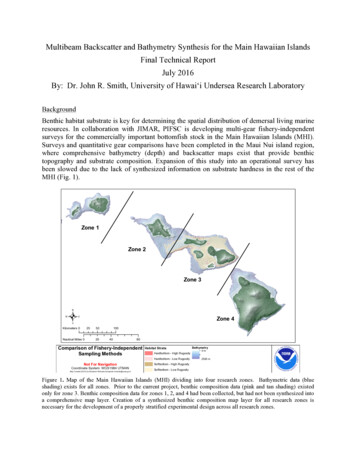
Multibeam Backscatter and Bathymetry Synthesis for the Main Hawaiian IslandsFinal Technical ReportJuly 2016By: Dr. John R. Smith, University of Hawai‘i Undersea Research LaboratoryBackgroundBenthic habitat substrate is key for determining the spatial distribution of demersal living marineresources. In collaboration with JIMAR, PIFSC is developing multi-gear fishery-independentsurveys for the commercially important bottomfish stock in the Main Hawaiian Islands (MHI).Surveys and quantitative gear comparisons have been completed in the Maui Nui island region,where comprehensive bathymetry (depth) and backscatter maps exist that provide benthictopography and substrate composition. Expansion of this study into an operational survey hasbeen slowed due to the lack of synthesized information on substrate hardness in the rest of theMHI (Fig. 1).Zone 1Zone 2Zone 3.Zone 4Kilometers 025Nautical Miles 050201004080Comparison of Fishery-IndependentSampling MethodsHabitat StrataHardbottom - High RugosityHardbottom - Low RugosityNot For NavigationCoordinate System: WGS1984 UTM4NMap Created (2013) by Benjamin Richards (benjamin.richards@noaa.gov)Bathymetry0m2500 mSoftbottom - High RugositySoftbottom - Low RugosityFigure 1. Map of the Main Hawaiian Islands (MHI) dividing into four research zones. Bathymetric data (blueshading) exists for all zones. Prior to the current project, benthic composition data (pink and tan shading) existedonly for zone 3. Benthic composition data for zones 1, 2, and 4 had been collected, but had not been synthesized intoa comprehensive map layer. Creation of a synthesized benthic composition map layer for all research zones isnecessary for the development of a properly stratified experimental design across all research zones.
In order to conduct a comprehensive, robust multi-gear fishery-independent survey for the MHIbottomfish stock, it is important to have maps of water depth, benthic topography, and substratecomposition which are known to structure the population densities and community compositionof ecological communities (Richards et al., 2012). The study referenced above developed andvalidated a six-point stratification based depth (75-200m, 200-400m), benthic slope (0 -20 , 20 90 ) and substrate composition (hard bottom, soft bottom), and synthesis data for the first twofactors already exist for the MHI sampling domain.The multibeam backscatter data necessary to resolve substrate composition for the MHI domainhave been collected, but with a variety of sensors operating at a range of different frequencies,such that similar numeric values from disparate areas do not signify similar levels of substratehardness. The lack of readily available backscatter synthesis products across the MHI surveydomain is an impediment to the development of a properly stratified operational fisheryindependent survey for MHI bottomfish.ObjectivesIn collaboration with partners at the University of Hawai‘i Undersea Research Laboratory(HURL), JIMAR conducted a one-year habitat assessment to address the lack of an integratedbenthic habitat mapping of the MHI. The project objectives were to:1. Create a synthesized benthic habitat substrate characterization (hard or soft bottom) with 20 mresolution from existing backscatter data in the Main Hawaiian Islands extending from theshoreline to a depth of 400 m;2. Develop a synoptic survey stratification and sampling allocation for the MHI survey domainusing the newly created MHI benthic substrate composition synthesis in combination withexisting bathymetric and topographic products as well as a stratified variance structure forMHI bottomfish resources for implementation of a fishery-independent survey of demersalfishery resources.Only objective #1 is discussed within this report.ApproachBackscatter data have been collected and archived for virtually all of the Main Hawaiian Islandsat depths from 100 to 400 m and to a lesser extent from the shoreline down to 100 m. Separatedata sets have been collected from a number of ships at different times and spatial scales, using avariety of multibeam systems. Recently, a protocol using GIS tools has been resolved andapplied. Basically, backscatter values from these data sets were reprocessed and standardized toa uniform scale of intensity. This protocol was used to create a 60 m resolution backscattersynthesis of the entire Main Hawaiian Islands seafloor to abyssal depths (Kelley and Smith,2014). For this project, the method was applied to create a higher resolution 5 m backscattersynthesis for the 75 to 400 m depth range that provides the benthic habitat substratecharacterization needed for bottomfish studies. A corresponding 5 m multibeam bathymetrysynthesis was also developed and used to correct the backscatter data for topographic slope. Thedepth range for both products extends from as shallow as data were available to at least 500 mand much deeper in some portions of the project area.2
Figure 2. Bathymetry and topography of the Main Hawaiian Islands with variously colored lines delineating theindividual grid boxes used for this study as discussed in the text.Data sets incorporated into the synthesesIn order to generate grids of the backscatter and bathymetry syntheses at 5 m cell size, eachresearch zone depicted in Fig. 1 was further broken up into smaller grid boxes (Fig. 2). This wasdone to speed up gridding, remain within computer memory limits, and simplify datamanagement for the numerous multibeam input files. This resulted in three boxes for Kaua‘iCounty, three for Honolulu County (O‘ahu), nine for Maui County and Penguin Bank (MauiNui), and four for Hawai‘i County (Big Island) for a total of 19. The individual grids were thenmerged into one grid for each county, and eventually into one grid for the entire chain.Modern multibeam systems collect coincident bathymetry and backscatter data that areincorporated into the same file or file system. By simply manipulating options in the postprocessing software, either component can be further processed, edited, gridded, plotted, and/ormerged with other like data. Older multibeam systems only collect bathymetry data. To furthercomplicate the issue, not all backscatter data are of equal quality and scaling, and thus cannot bemeaningfully and directly merged with such data from other ships, systems, and/or frequencies.While the quality and resolution of multibeam bathymetry data also vary between differentinstallations, these data can be meaningfully and directly combined, although one usuallyemploys weighting factors to produce the best result.A total of 34,618 individual multibeam bathymetry files from hundreds of cruises traversing theMain Hawaiian Islands were interrogated to see if they would contribute bathymetric coverage toeach of the 19 grid boxes discussed above. The contributing files were then incorporated into amuch smaller list with appropriate weighting and gridding was accomplished. The number offiles used in each grid varied considerably depending on number of surveys or opportunistic3
transits crossing the grid box, systems used and extent of water depth ranges, the latter twofactors affecting track line spacing. Using all data available (unless it contained obviousartifacts) allowed the creation of complete grids with limited data gaps where there were nomultibeam data available. Regarding the backscatter synthesis, files were selectively chosenmanually and only dedicated surveys, as opposed to opportunistic transits, were included unlessa gap in coverage needed filling. This allowed for the highest quality product and was necessaryto reduce the manual workload.Sensors and research teams that produced the original data setsBackscatter data acquired with the following systems and vessels were used in the project:Kongsberg EM 120 [12 kHz], R/V Kilo MoanaKongsberg EM 122 [12 kHz], R/V Kilo MoanaKongsberg EM 300 [30 kHz], M/V Ocean Alert, NOAA Ship Hi‘ialakaiKongsberg EM 302 [30 kHz], NOAA Ship Okeanos Explorer, R/V FalkorKongsberg EM 710 [40 – 100 kHz], R/V Kilo Moana, R/V FalkorKongsberg EM 1002 [95 kHz], R/V Kilo MoanaKongsberg EM 3002d [300 kHz band], NOAA Ship Hi‘ialakaiReson 8101-ER [240 kHz], R/V AHI (30 ft shallow draft boat for near shore work)Bathymetry data acquired with these and other multibeam systems and ships were used,including SeaBeam classic, SeaBeam 2000, SeaBeam 2112, Hydrosweep, and LIDAR.The organizations who carried out and/or funded these surveys included, but were not limited to:University of Hawai‘i Undersea Research Laboratory and the Hawai‘i Mapping Research GroupU.S. Geological Survey (USGS), Western Coastal and Marine Geology ProgramNOAA/PIFSC Coral Reef Ecosystem Division, Pacific Islands Benthic Habitat Mapping CenterNOAA Undersea Research Program and the Office of Ocean Exploration and Research (OER)NOAA Pacific Islands Regional Office (PIRO)Monterey Bay Aquarium Research Institute (MBARI)Schmidt Ocean Institute (SOI)Methods used to produce the synthesesBathymetryWhen available, edited versions of the original multibeam “swath files” (collected by the sonarsystems) were used in the bathymetry gridding schemes. These data were edited by the surveyteams while aboard ship and/or sometime afterwards ashore using a variety of open source andcommercial software including, but not limited to, MB-System, SABER, Caris, and Fledermaus.When edited data were not available, the files were typically assigned a low weighting so thatbetter quality data would take precedence in the grid. The same idea applied for dedicatedversus opportunistic transit survey data. Further editing of bathymetry data was beyond thescope of this project, although time was spent investigating obvious artifacts, determining theoffending files, removing them from the data lists, and then rerunning the gridding process.4
Gridding of the bathymetry component was exclusively carried out using the MB-System(Caress and Chayes, 1995, 1996) and Generic Mapping Tools (GMT) (Wessel and W. Smith,1991) open source software packages. These are community standards and are run from thecommand line or in job scripts in a Unix/Linux shell. Examples of the gridding and filteringcommands, respectively, are provided below.mbgrid -E5.0/5.0m! -F1 -A2 -C10 -I datalist1 -N -O outgrid -R range1-V -JU -S7grdfilter outgrid -G filtgrid -D0 -Fm50Once all 19 final bathymetry grids were run, they were fused into grids for each county, and thenfurther merged into one grid for the entire Main Hawaiian Island chain (Fig. 3).Figure 3. Five-meter resolution multibeam bathymetric synthesis for the Main Hawaiian Islands with islandtopography in gray shades. Cooler colors (i.e., blue) indicate shallow depths, while hotter colors (i.e., red) indicateshallow depths.BackscatterBackscatter processing was generally carried using the raw swath files in most instances. Thereasons for this were to create a more consistent product across surveys, systems, and ships, andto employ the open source Geocoder software module (embedded in in the commercial QPS’sFledermaus/FMGT software package). This is a relatively new technique and had not beenapplied to any of the existing data to the best of our knowledge. However, for multibeam data,FMGT will only accept raw.all or certain Generic Sensor Format (GSF) files and not the edited5
bathymetry files. Thus, to compensate for bathymetric data artifacts, filtered bathymetry“reference” grids were read into the FMGT project to correct the backscatter data. FMGT is alsofar more sensitive to corrupted or missing data or metadata in the files, along with being morememory limited than MB-System programs. As a result, FMGT will crash repeatedly when itencounters a significant error, or refuse to begin processing until memory issues are addressed.After the metadata are extracted, FMGT computes the coverage and extracts the navigation ofeach line. In all but one case, the default settings for FMGT were used in processing thebackscatter data. The software reads the swath files’ metadata and automatically adjusts theprocessing scheme to produce the best result. The metadata contains information such asgeographic extents, datagram packet numbers, sonar modalities, and sonar type. The oneexcursion from the default values occurred when processing EM 1002 data from R/V KiloMoana. Here, the Backscatter Source was changed from the default Beam Time Series to BeamAverage (calibrated) in order to produce a more consistent result, or look, for the entire survey.The following statements regarding the processing steps carried out in FMGT are paraphrasedfrom the online Fledermaus Reference Manual (2016). FMGT first adjusts the backscatter databy extracting the backscatter then executing radiometric corrections based on sonar type andbottom topography. Next, it performs filter processing that includes angle varying gain (AVG)adjustments along with anti-aliasing of the backscatter data. As this stage advances, it transmitsthe results of the backscatter adjustment to the project hierarchy. Finally, FMGT builds thedesired mosaic using the pre-calculated or manually assigned resolution. This value is precomputed by FMGT during coverage processing and is estimated based on the sonar beamconfiguration and along track coverage. For this project, all data set resolution estimates wereoverridden and manually assigned the value of 5 m. At this point, interactive manipulation oftoggling off files because of turns, data artifacts, or overlapping swaths occurred. The mosaicswere then re-rendered and output to ArcGIS grids for incorporation into the next phase of theprocess (Fig. 4). Data from identical multibeam systems and ships (and multiple cruises of sameship) were processed and combined into the same mosaic and resultant grid.The surveys (files) that could not be read into FMGT were processed using the mbgrid module ofMB-System. This method allows the manual setting of various options and does not read the filemetadata to automatically optimize the processing options and flow. The result is a “rougher”look, including more noticeable nadir artifacts that do cause more false “hard bottom”classification. However, the program is extremely robust – able to read, process, and grid nearlyevery available sonar system format. Jobs can be batched and run autonomously once theoptions are chosen, leading to a high degree of computational efficiency. Example commandlines using MB-System for backscatter gridding and conversion to ArcGIS format, respectively,are given below. Again, single system, single ship, multiple cruises, and then the resultant gridsfrom this package were ready for import into ArcGIS to accomplish the next processing steps(Fig. 4).mbgrid -E5.0/5.0m! -F1 -A4 -JU -C5 -U5 -N –I datalist2 –O outgrid -V–R range2mbm grd2arc -V –I outgrid –O arcgrid6
ESRI ArcGIS is where the magic happened. An outline of the major processing steps is givenbelow, using Ni‘ihau as an example, followed by a more detailed description of the criticalreclassification procedure.Figure 4. Backscatter data around Ni‘ihau. Brown color indicates harder seafloor, while yellow/gold denotes softerseafloor. Left side image is a stack of five ‘raw’ data sets. Right side are same data sets after going throughreclassification and synthesizing process described in text and depicted in following figures.Figure 5. Three examples from Ni‘ihau the data sets showing how the histograms from the raw grids (gray) areadjusted (magenta) in ArcGIS by using the sliders on top and bottom of graph. X-axis is backscatter value, Y-axis ispixel count. See Fig. 6 for more examples and explanation.We converted the ASCII grids to rasters (floating point), defined the projection (UTM zone 4N),generated a histogram and manually trim the upper and lower tails (Fig. 5), then compared theresult to other grid layers already imported and reclassified. Iterated as necessary. This is one oftwo mostly subjective steps in the process. When satisfied with the look of the backscatter matchbetween grid layers in the display, the reclassify tool was then used to apply the reclassification7
Figure 6. Histograms extracted from all five data sets making up the Ni‘ihau mosaic, as shown in Fig. 4. Leftcolumn shows raw grids prior to reclassification, and afterwards (right column). The multibeam systems and vesselsare indicated on right side, and were mosaicked in this order, from top to bottom. The red lines labeled 140 showsthe position of the chosen threshold hard-soft value on each reclassified histogram. Note the wide range ofbackscatter values on the X-axis within the left column and how they become standardized in right column.8
values to the grid itself, rather than just to the display (Fig. 6). One caveat must be noted here.The reclassification back to grid feature was disabled by ESRI after ArcGIS version 10.0. Innewer versions, it only operates on the display, thus we have maintained one softwareinstallation of ArcGIS 10.0 simply to allow use of this feature for backscatter synthesizing.After properly ordering the stack of grid layers (generally best data on top, worst on bottom), thefinal step in the process was to generate a combined mosaic for the grid box by using the Mosaicto New Raster tool (Fig. 7). The same tool was later used to produce mosaics for entire counties(island groups) and the whole main island chain (Fig. 8).The reclassification step, also referred to as outlier adjustment, is the critical and also thesubjective stage of this method. It allows the user to visually adjust usually overlappingbackscatter grid layers produced with data from different multibeam systems so that they have asimilar, if not identical look. This is regardless of the actual numerical range of the original gridvalues, which get rescaled to an imagery standard of 1 to 256. This actually happens twice, firstwhen brought into ArcGIS, but remains only in the display. Adjusting the histograms reassignsthe 1 to 256 range to the new, trimmed histogram, also still in the display only until one entersthe Reclassify tool and applies the changes to the actual grid values.Figure 7. Final histogram of the five reclassified and synthesized Ni‘ihau data sets with the 140 threshold indicatedby red line and label. Note the appearance of overlapping histograms within the same range of values and a moreGaussian shape overall. In this case, there is somewhat of a notch in the histogram at the breakpoint of 140.Interpretation of the dataThe next stage in the process (also the second mostly subjective step) was developing thethreshold-based hard/soft categorization, or breakpoint value. From this, an interpretative9
substrate map delineating hard and soft bottom values could be generated. This interpretativephase was based on the initial work done by Dr. Christopher Kelley of UH/HURL on theassemblage of disparate backscatter data sets. He worked primarily with the USGS and MBARIsurvey data using the EM 300 data from M/V Ocean Alert to determine hard/soft transitionsbased on ground-truthing in the form of video observations from the HURL Pisces submersibles.Here, he chose a threshold value of 187 and greater (out of 1 to 256) which was independentlyderived by Dartnell and others (2006) based on work using the same system from the samevessel offshore California.Figure 8. Final five-meter resolution multibeam backscatter synthesis for the Main Hawaiian Islands with islandtopography in gray shades. Brown color indicates harder seafloor, while yellow/gold denotes softer seafloor.While the 187 value provided a starting point for this study, it was realized that the hard/softvalue would not be the same for the synthesized data sets because of the reclassification requiredto merge them into one coherent grid. This lead to the analysis of histograms for the reclassifiedEM 300 data for Maui Nui, where we found an obvious breakpoint in one histogram with a valueof 146. The next step involved building layers displaying only values of 146 to 256 for thereclassified and synthesized data sets for the other counties. Additional layers were generatedwith values of 130, 135, 140, 141 (all to 256) and repeatedly compared with the “original” 187 to256 data sets to determine which threshold value from the new syntheses most closely matchedthe original value and/or best represented the delineation of hard versus soft bottom. We alsoconsidered how known data artifacts may skew the threshold value. Potential variability of thereclassified syntheses between counties was also examined. In the end, a single best-fit thresholdvalue of 140 was chosen for all counties, and at this point the four different backscatter mosaicswere fused into one final grid representing the entire Main Hawaiian Island chain (Fig. 9).10
Figure 9. Final five-meter resolution hard-soft grid for the MHI derived from the backscatter synthesis exhibited inFig. 8. All values from 140-256 are red (hard bottom), those 0-139 are tan (soft bottom).Verification of accuracyRegarding the bathymetry synthesis, much care was taken during its build to examine, identify,and ferret out individual files with bad data that created noticeable artifacts when compiled.Fortunately, there were usually enough overlapping surveys and data swaths in the archive thatwe had the luxury of toggling off obviously bad sources and/or low-weighting inferior data, andstill had sufficient coverage to produce contiguous bathymetry grids. For the backscattersynthesis, survey geometry and quality were considered when choosing the surveys/files toinclude. We also carefully evaluated in what order the data sets for each area should be stacked,based on system capability, installation quality, available coverage, processing algorithm used(FMGT vs. MB-System), and consistency of the reclassification results with other data sets. Asa result, the backscatter layer stack order changed slightly or greatly for each mosaicked area toproduce the best and most uniform product.Ideally, one would compare the new hard-soft bottom grid directly with ground-truth data fromsubmersibles, ROVs, towed/drop cameras, substrate samplers, etc. taken from a wide variety oflocations, geomorphologies, and water depths throughout the Main Hawaiian Islands. However,this task was beyond the scope of the project. Therefore, in addition to the exercise comparingour results with the previous 187 categorization described in the preceding section, we also didspot checking of our ‘140 layer’ with the full-value-range backscatter synthesis and bathymetrysynthesis produced as part of this study. In general, the hard (high) values correspond withexpected geologic and morphologic features such as reef terraces, steep scarps, debris channels11
with coarse sediment, exposed lava flows and cones, current swept surfaces, headlands,submarine canyon walls, and carbonate platforms. Soft values (low) values demarcate featuresincluding sediment basins and other catchments, low-slope abyssal seafloor, and nearshore areasin close proximity to high terrestrial runoff.Known issuesSome known issues, also referred to as data artifacts in this report, warrant identification andfurther explanation for potential users of these products. Attempts were indeed made duringprocessing to diminish their manifestation. Additionally, some comments are presentedregarding how the effect of the artifacts on these products can be minimized during use.Figure 10. Close-up view of backscatter data off the northeastern end of Ni‘ihau showing three different artifacts:nadir lines (indicated by black rectangles), variable power/gain (blue polygon), on-land chatter (ellipses). See textfor explanation and Fig. 4 for location.12
Several different artifacts are highlighted in Figs. 10 and 11. The black boxes show nadirartifacts. Nadir lines in backscatter basically represent the ship track and is the portion directlyunder the vessel where no useable backscatter are acquired since this data type relies on slantrange sonar returns. As a result, the nadirs appear darker than the data from the rest of the swathto either side of the ship. More sophisticated processing and filtering algorithms can remove orat least subdue, many of the nadir artifacts. When possible, FMGT/Geocoder was used in thisproject to process the backscatter data, which did a good job of blending the nadirs. Geocoderfailed on several of the data types, including Hi‘ialakai (EM 300, EM 3002), USGS 1998 datafrom Ocean Alert (EM 300), and AHI (Reson 8101). In these cases, MB-System (mbgrid) wasutilized which is more robust but has less complexity in its processing and options.Figure 11. Close-up view of backscatter data off the northwestern side of the Big Island of Hawai‘i showing nadirartifacts (indicated by black rectangles). See text for further explanation and inset map for location.The blue box in Fig. 10 shows a probable automatic power and/or gain increase in one of theshallow/intermediate multibeam systems operating near its depth limit (e.g., Kilo Moana's EM1002). Some of these show up in waters deeper than 500 m, well below the bottomfish range ofinterest and thus beyond the boundaries of the synoptic survey stratification grid cells. Thecircled artifacts in Fig. 11 that overlap the terrestrial domain resulted from processing the AHIbackscatter data in MB-System’s mbgrid. In some cases with AHI Reson 8101 data, Geocodercould be used and such artifacts did not appear, although with the larger data sets, such as atNi‘ihau, it crashed repeatedly. Again, the depth range in which these artifacts occur is beyond(above) the depth range of interest for which this project was developed. Creating a mask using13
the bathymetry and/or topography to exclude the artifacts is another method that could beimplemented to lessen their effects.Finally, while high slopes generally will produce strong returns in backscatter suggesting a hardbottom, in reality, this is not always the case. It really depends on the survey geometry. In somecases, one has to drive the ship into the same steep area from numerous angles just to get somecoverage because of the high slope. If the slope is facing 'away' from the swath, little to noacoustic return will be received. Likewise, even if the ship is navigating along an ideal headingto map the morphology, extremely steep slopes can cause shadowing of the fan-shaped swathdownslope, leaving gaps in both the bathymetric and backscatter data. Repeated passes fromadjacent lines are the only way to achieve more complete coverage, at the expense of more shiptime! For more extensive discussion of multibeam backscatter acquisition, processing andinterpretation, the interested reader is referred to Lurton and Lamarche (2015).Education and outreach activitiesEducation and outreach activities were not incorporated into the proposed project. However, anumber of entities requested use of the data products during the course of the effort. Theseincluded a doctoral student at the UH/HIMB using it for modeling mesophotic hard coraldistribution across the Main Hawaiian Islands, the State of Hawai‘i DLNR/DAR to assemble ageodatabase for bottomfish management use, a film production group from the UK doing adocumentary for National Geographic, and the NOAA Office of Exploration and Research foruse as base maps for ROV dives from Okeanos Explorer.AcknowledgementsThe NOAA/PIFSC Fisheries Research and Monitoring Division (FRMD), through a grant toJIMAR, provided funding from for this project. Special thanks go to Dr. Annie Yau and Dr.Benjamin Richards of PIFSC and the FRMD Stock Assessment Program who oversaw andcollaborated on this project. Dr. Christopher Kelley of UH/HURL originally developed thebackscatter reclassification and synthesizing technique for a previous study. He and Ms.Virginia Moriwake of the SOEST/University of Hawai‘i provided valuable advice, technicalassistance, and collegial support for the duration of this project. This work also benefited fromthe use of computer workstations donated by Hewlett-Packard and Intel to UH/HURL.ReferencesCaress, D. W. and D. N. Chayes (1996), Improved Processing of Hydrosweep Multibeam Dataon the R/V Maurice Ewing, Marine Geophysical Researches, 18: 631-650.Caress, D. W., and D. N. Chayes (1995), New software for processing sidescan data fromsidescan-capable multibeam sonars, Proceedings of the IEEE Oceans 95 Conference, 9971000, 1995.Dartnell, P., B. D. Edwards, E. L. Phillips, D. E. Montagne, D. B. Cadien, and G. Robertson(2006), An Empirical Approach to Mapping the Distribution of Seafloor Geologic andBiologic Characteristics Offshore San Pedro, Southern California, Eos Trans. AGU, 87(36),Ocean Sci. Meet. Suppl., Abstract OS15F-11.14
Fledermaus Reference Manual (online) (2016). https://confluence.qps.nl/display/FM760/Kelley, C.D. and J.R. Smith, Regional multibeam backscatter synthesis of the Main HawaiianIslands at 60 m resolution backscatter.phpLurton, X. and G. Lamarche (editors) (2015),Backscatter measurements by seafloor-mappingsonars - Guidelines and Recommendations. A collective report by members of the GeoHabBackscatter Working Group.https://www.niwa.co.nz/static/BWSG REPORT MAY2015 web.pdfRichards, B. L., Williams, I. D., Vetter, O. J., & Williams, G. J. (2012), Environmental FactorsAffecting Large-Bodied Coral Reef Fish Assemblages in the Mariana Archipelago, PLoSONE, 7(2), e31374, doi:10.1371/journal.pone.0031374.Wessel, P. and W. H. F. Smith (1991), Free software helps map and display data, EOS Trans.AGU, 72, 441.Contact InformationJohn R. Smith, Ph.D.Oceanographer (MG&G)Science DirectorHawai‘i Undersea Research Laboratoryat SOEST/University of Hawai‘i1000 Pope Road, MSB 229Honolulu, HI 96822Tel: 808-956-9669E-mail: jrsmith@hawaii.eduwww.soest.hawaii.edu/HURL15
Map of the Main Hawaiian Islands (MHI) dividing into four research zones. Bathymetric data (blue shading) exists for all zones. Prior to the current project, benthic composition data (pink and tan shading) existed only for zone 3. Benthic composition data for zones 1, 2, and 4 had been collected, but had not been synthesized into