Transcription
Computational advances in polynomial optimization: RAPOSa,a freely available global solverBrais González-Rodríguez 1 , Joaquín Ossorio-Castillo3 , Julio González-Díaz1,3 , ÁngelM. González-Rueda2 , David R. Penas1 , and Diego Rodríguez-Martínez31 Departmentof Statistics, Mathematical Analysis and Optimization, MODESTYA Research Group and IMAT,University of Santiago de Compostela.2 Department of Mathematics, MODES Research Group and CITIC, University of A Coruña.3 ITMATI (Technological Institute for Industrial Mathematics).July 31, 2021AbstractIn this paper we introduce RAPOSa, a global optimization solver specifically designed for (continuous) polynomial programming problems with box-constrained variables. Written entirely in C ,RAPOSa is based on the Reformulation-Linearization Technique developed by Sherali and Tuncbilek(1992) and subsequently improved in Sherali et al. (2012a), Sherali et al. (2012b) and Dalkiranand Sherali (2013). We present a description of the main characteristics of RAPOSa along witha thorough analysis of the impact on its performance of various enhancements discussed in theliterature, such as bound tightening and SDP cuts. We also present a comparative study withthree of the main state-of-the-art global optimization solvers: BARON (Tawarmalani and Sahinidis,2005), Couenne (Belotti et al., 2009) and SCIP (Achterberg, 2009).Keywords Global optimization, Polynomial programming, Reformulation-Linearization Technique(RLT).1IntroductionIn this paper we introduce RAPOSa (Reformulation Algorithm for Polynomial Optimization Santiago), a new global optimization solver specifically designed for polynomial programming problems with box-constrained variables. It is based on the Reformulation-Linearization Technique (Sherali and Tuncbilek, 1992), hereafter RLT, and has been implemented in C . Although it is not opensource, RAPOSa is freely distributed and available for Linux, Windows and MacOS. It can also berun from AMPL (Fourer et al., 1990) and from NEOS Server (Czyzyk et al., 1998). The RLT-basedscheme in RAPOSa solves polynomial programming problems by successive linearizations embeddedinto a branch-and-bound scheme. At each iteration, a linear solver must be called, and RAPOSa hasbeen integrated with a wide variety of linear optimization solvers, both open source and commercial,including those available via Google OR-tools (Perron and Furnon, 2019). Further, auxiliary callsto nonlinear solvers are also performed along the branch-and-bound tree to improve the performanceof the algorithm, and again both open source and commercial solvers are supported as long as theycan be called from .nl files (Gay, 1997, 2005). More information about RAPOSa can be found athttp://www.itmati.com/RAPOSa/index.html.In conjunction with the introduction of RAPOSa, the other major contribution of this paper is tostudy the impact of different enhancements on the performance of the RLT. We discuss not only theindividual impact of a series of enhancements, but also the impact of combining them. To this end,Section 4 and Section 5 contain computational analyses on the use of J-sets (Dalkiran and Sherali,2013), warm starting of the linear relaxations, changes in the branching criterion, the introduction ofbound tightening techniques (Belotti et al., 2009, 2012; Puranik and Sahinidis, 2017) and the additionof SDP cuts (Sherali et al., 2012a), among others. Interestingly, RAPOSa incorporates a fine-grained braisgonzalez.rodriguez@usc.es.1
distributed parallelization of the branch-and-bound core algorithm, which delivers promising speedupsas the number of available cores increases.The most competitive configurations of RAPOSa according to the preceding extensive analysis arethen compared to three popular state-of-the-art global optimization solvers: BARON (Tawarmalani andSahinidis, 2005), Couenne (Belotti et al., 2009) and SCIP (Achterberg, 2009). The computationalanalysis is performed on two different test sets. The first one, DS-TS, is a set of randomly generatedpolynomial programming problems of different degree introduced in Dalkiran and Sherali (2016) whenstudying their own RLT implementation: RLT-POS.1 The second test set, MINLPLib-TS, containsthe polynomial programming problems with box-constrained and continuous variables available inMINLPLib (Bussieck et al., 2003). The main results can be summarized as follows: i) In DS-TS,all configurations of RAPOSa clearly outperform BARON, Couenne and SCIP, with the latter performingsignificantly worse than all the other solvers and ii) In MINLPLib-TS, differences in performance aresmaller across solvers, with SCIP exhibiting a slightly superior performance. Importantly, the enhancedversions of RAPOSa are clearly superior in this test set to the baseline configuration.The outline of the paper is as follows. In Section 2 we present a brief overview of the classic RLTscheme and different enhancements that have been introduced in recent years. In Section 3 we discusssome specifics of the implementation of RAPOSa and of the testing environment. In Section 4 we presentsome preliminary computational results, in order to define a configuration of RAPOSa that can be usedas the baseline to assess the impact of the main enhancements, discussed in Section 5. In Section 6 wepresent the comparative study with BARON, Couenne and SCIP. Finally, we conclude in Section 7.22.1RLT: State of the art and main contributionsBrief overview of the techniqueThe Reformulation-Linearization Technique was originally developed in Sherali and Tuncbilek(1992). It was designed to find global optima in polynomial optimization problems of the followingform:minimize φ0 (x)subject to φr (x) βr , r 1, . . . , R1(1)φr (x) βr , r R1 1, . . . , Rnx Ω R .where N {1, . . . , n} denotes the set of variables, each φr (x) is a polynomial of degree δr N,Ω {x Rn : 0 lj xj uj , j N } Rn is a hyperrectangle containing the feasibleregion, and the degree of the problem is defined as δ maxr {0,.,R} δr .A multiset is a pair (S, p), in which S is a set and p : S N is a map that indicates the multiplicityof each element of S. We slightly abuse notation and use (N, δ) to denote the multiset of variables(N, p) in whichp(i) δ for each i N . For each multiset (N, p), its cardinality is defined byP (N, p) i N p(i).The RLT algorithm involves two main ingredients. First, the bound-factor constraints, given, foreach pair of multisets J1 and J2 such that J1 J2 (N, δ) and J1 J2 δ, byYYFδ (J1 , J2 ) (xj lj )(uj xj ) 0.(2)j J1j J2Note that any point in Ω satisfies all the bound-factor constraints. Second, the RLT variables, given,for each multiset J (N, δ) such that 2 J δ, byYXJ xj .(3)j JNote that each multiset J can be identified with a monomial. For instance, the multiset J {1, 1, 2, 3, 4, 4} refers to the monomial x21 x2 x3 x24 . Therefore, to each monomial J one can associatedifferent bound factors of the form J J1 J2 , depending on which variables are used for the lowerbound factors and which ones for the upper-bound factors. Further, monomial J {1, 1, 2, 3, 4, 4} alsodefines the RLT variable X112344 .1 Unfortunately, we could not include RLT-POS in our comparative study, since this implementation is not publiclyavailable.2
The first step of the RLT algorithm is to build a linear relaxation of the polynomial problem (1).To do this, the polynomials of the original problem are linearized by replacing all the monomials withdegree greater than 1 by their corresponding RLT variable (3). This linearization is denoted by [·]L .Furthermore, the linearized bound-factor constraints in (2) are added to get tighter linear relaxations:minimize [φ0 (x)]Lsubject to [φr (x)]L βr ,r 1, . . . , R1[φr (x)]L βr ,r R1 1, . . . , R[Fδ (J1 , J2 )]L 0, J1 J2 (N, δ), J1 J2 δx Ω Rn .(4)Note that if constraints in (3) are added to the linear relaxation (4), the resulting problem isequivalent to problem (1). The next step of the RLT algorithm is to solve the linear relaxation in (4)to obtain a lower bound of the original polynomial problem. Next, a branch-and-bound scheme is usedto find the global optimum of the polynomial problem. Since a solution of the linear relaxation thatsatisfies constraints in (3) is feasible to problem (1), the branching rule is usually based on violationsof these constraints, which are referred to as RLT-defining identities. The convergence of this schemeto a global optimum is proven in Sherali and Tuncbilek (1992).Along the branch-and-bound tree, the RLT algorithm obtains, and gradually increases, lowerbounds for the optimal solution of the minimization problem by solving the linear relaxations. Itobtains upper bounds when the solution of a linear relaxation is feasible in the original problem. Theabsolute and relative differences between the lower and upper bounds lead to the so called absolute andrelative optimality gaps. The goal of the algorithm is to close these gaps to find the global optimumof the polynomial problem. Thus, stopping criteria often revolve around thresholds on the optimalitygaps.2.2Enhancements of the original RLT algorithmIn this section we briefly discuss six enhancements of the basic RLT algorithm. All of them arepart of the current implementation of RAPOSa and its impact on the performance of the algorithm isthoroughly analyzed in Section 4 and Section 5.2.2.1J -setsThis enhancement was introduced in Dalkiran and Sherali (2013), where the authors prove that itis not necessary to consider all the bound-factor constraints in the linear relaxation (4). Specifically,they prove two main results. The first one is that convergence to a global optimum is ensured even ifonly the bound-factor constraints associated with the monomials that appear in the original problemare included in the linear relaxation. The second result is that convergence to a global optimum is alsoensured without adding the bound-factor constraints associated with monomials J J 0 , provided thebound-factor constraints associated with J 0 are already incorporated. Equipped with these two results,the authors identify a collection of monomials, which they call J-sets, such that convergence to a globaloptimum is still guaranteed if only the bound-factor constraints associated with these monomials areconsidered.The use of J-sets notably reduces the number of bound-factor constraints in the linear relaxation (4)(although it still grows exponentially fast as the size of the problem increases). The main benefit ofthis reduction is that it leads to smaller LP relaxations and, hence, the RLT algorithm requires lesstime in each iteration. The drawback is that the linear relaxations become less tight because they haveless constraints and more iterations may be required for convergence. Nevertheless, practice has shownthat the approach with J-sets is clearly superior. We corroborate this fact in the numerical analysisSection 4.1.2.2.2Use of an auxiliary local NLP solverMost branch-and-bound algorithms for global optimization rely on auxiliary local solvers and theRLT scheme can also profit from them, as already discussed in Dalkiran and Sherali (2016). Theyproposed to call the nonlinear local solver at certain nodes of the branch-and-bound tree. In each call,the nonlinear local solver is provided with an initial solution, which is the one associated to the lowerbound of the RLT algorithm at that moment.3
This strategy helps to decrease the upper bound more rapidly and, hence, allows to close theoptimality gap more quickly. The only drawback is the time used in the call to the nonlinear solver.Practice has shown that, in general, it is beneficial to call it only at certain nodes instead of doing soat each and every node.2.2.3Products of constraint factors and bound factorsThis enhancement was already mentioned in Sherali and Tuncbilek (1992) when first introducingthe RLT technique for polynomial programming problems. It consists of defining tighter linear programming relaxations by strengthening constraint factors of the form φr (x) βr 0 of degree lessthan δ. More precisely, one should take products of these constraint factors and/or products of boundfactors in such a way that the resulting degree is no more than δ. Similar strengthenings can also beassociated to equality constraints φr (x) βr of degree less than δ, by multiplying them by variablesof the original problem.Note that, although the new constraints are tighter than the original ones in the nonlinear problem,this is not necessarily so in the linear relaxations. Thus, we also preserve the original constraints toensure that the resulting relaxations are indeed tighter and, therefore, the lower bound may increasemore rapidly. Since the addition of many of these stronger constraints may complicate the solution ofthe linear relaxations, one should carefully balance these two opposing effects.2.2.4Branching criterionThe design of a branch-and-bound algorithm requires to properly define different components ofthe algorithm. The most widely studied ones are the search strategy in the resulting tree, pruning rulesand branching criterion; refer, for instance, to Achterberg et al. (2005) and Morrison et al. (2016). InSection 5.4 we focus on the latter of these components. More precisely, we study the impact of thecriterion for the selection of the branching variable on the performance of the RLT technique.2.2.5Bound tighteningBound tightening techniques are at the core of most global optimization algorithms for nonlinearproblems (Belotti et al., 2009, 2012; Puranik and Sahinidis, 2017). These techniques allow to reducethe search space of the algorithm by adjusting the bounds of the variables of the problem. Two mainapproaches have been discussed in the literature: i) Optimality-based bound tightening, OBBT, inwhich bounds are tightened by solving a series of relaxations of minor variations of the original problemand ii) Feasibility-based bound tightening, FBBT, in which tighter bounds are deduced directly byexploring the problem constraints. Since OBBT is computationally demanding while FBBT is not,combined schemes are often used, under which OBBT is only performed at the root node and FBBTis performed at each and every node of the branch-and-bound tree.These techniques lead to tighter relaxations and, therefore, they do not only reduce the searchspace, but they also help to increase the lower bound of the optimization algorithm more rapidly.Moreover, since the resulting linear relaxations are not harder to solve than the original ones, boundtightening techniques are often very effective at improving the performance of global optimizationalgorithms.2.2.6SDP cutsThis enhancement is introduced in Sherali et al. (2012a) and consists of adding specific constraints,called positive semidefinite cuts, SDP cuts, to the linear relaxations generated along the branchand-bound tree. These constraints are built as follows. First, a matrix of the form M [yy T ] isdefined, where y can be any vector defined using variables and products of variables of the originalproblem. Since all the variables of the polynomial problem (1) are non-negative, matrix M is positivesemidefinite in any feasible solution. Therefore, given a solution of the current linear relaxation, wecan evaluate M at this solution, obtaining matrix M̄ . If this matrix is not positive semidefinite, thenwe can identify a valid linear cut to be added to the linear relaxation. More precisely, if there is avector α such that αT M̄ α 0, then constraint αT M α 0 is added to the linear relaxation.In Sherali et al. (2012a) this process is thoroughly explained and several strategies are discussed,such as different approaches to take vector y, different methods to find α and the number of cuts toadd in each iteration.4
3Implementation and testing environment3.1ImplementationEach execution of RAPOSa leans on two solvers: one for solving the linear problems generatedin the branch-and-bound process and one to compute upper bounds as mentioned in Section 2.2.2.The default (free) configuration of RAPOSa runs with Glop (B. De Backer, 2015) and Ipopt (Wächterand Biegler, 2006), although the best results are obtained using commercial solver Gurobi (GurobiOptimization, 2020) instead of Glop. Currently, RAPOSa supports the following solvers: Linear solvers: Gurobi (Gurobi Optimization, 2020), Glop (B. De Backer, 2015), CLP (LougeeHeimer, 2003) and lp solve (Berkelaar et al., 2004).2 Nonlinear local solvers: Ipopt (Wächter and Biegler, 2006), Knitro (Byrd et al., 2006), MINOS(Murtagh and Saunders, 1978) and CONOPT (Drud, 1985).RAPOSa has been implemented in C , and it is important to clarify that it connects differently tothe two types of solvers. Since solving the linear problems is the most critical part of the performance,it connects with the linear solvers through their respective C libraries. In the case of the nonlinearlocal solvers, the number of calls is significantly lower, and RAPOSa sends them an intermediate .nlfile with the original problem and a starting point.Importantly, the user does not need to explicitly generate .nl files to execute RAPOSa, since it canalso be run from an AMPL interface (Fourer et al., 1990).3 Moreover, RAPOSa can also be executed onNEOS Server (Czyzyk et al., 1998).3.2The testing environmentAll the executions reported in this paper have been performed on the supercomputer Finisterrae II,provided by Galicia Supercomputing Centre (CESGA). Specifically, we used computational nodespowered with 2 deca-core Intel Haswell 2680v3 CPUs with 128GB of RAM connected through anInfiniband FDR network, and 1TB of hard drive.Regarding the test sets, we use two different sets of problems. The first one is taken from Dalkiranand Sherali (2016) and consists of 180 instances of randomly generated polynomial programming problems of different degrees, number of variables and density.4 The second test set comes from the wellknown benchmark MINLPLib (Bussieck et al., 2003), a library of Mixed-Integer Nonlinear Programming problems. We have selected from MINLPLib those instances that are polynomial programmingproblems with box-constrained and continuous variables, resulting in a total of 168 instances. Hereafterwe refer to the first test set as DS-TS and to the second one as MINLPLib-TS.5All solvers have been run taking as stopping criterion that the relative or absolute gap is below thethreshold 0.001. The time limit was set to 10 minutes in comparisons between different configurationsof RAPOSa and to 1 hour in the comparison between RAPOSa and other solvers.4Preliminary results and RAPOSa’s baseline configurationThe goal of this section is to add to RAPOSa’s RLT basic implementation a minimal set of enhancements that make it robust enough to define a baseline version to assess, in Section 5, the impactof the rest of the enhancements. As we show below, the use of J-sets and an auxiliary nonlinearsolver are crucial in order to be able to get some success at tackling the problems in both DS-TS andMINLPLib-TS. Importantly, we also present in this section the results of a parallelized version of theRLT technique. However, it will not be part of the rest of the analysis in this paper since it would notallow for a fair comparison with the other solvers, which do not have these parallelization capabilities.The results in this section and in the following one are mainly illustrated by means of summarytables. Some comments are needed to explain the information shown in these tables; similar comments2 Theconnection with Glop and CLP was implemented using Google OR-tools (Perron and Furnon, 2019).B contains a short tutorial that explains how to interact with RAPOSa either directly with .nl files orthrough AMPL.4 By density we mean the proportion of monomials in the problem to the total number of possible monomials (giventhe degree of the problem).5 Instances from DS-TS can be downloaded at http://www.itmati.com/RAPOSa/files/DS-TS.zip and instances fromMINLPLib-TS can be downloaded at .3 Appendix5
apply to Table 10 in Section 6, where RAPOSa is compared with other global optimization solvers. Inthe row for the number of solved instances we show between brackets the number of instances solved byat least one configuration and the total number of instances in the corresponding test set. Regardingthe computation of both average and median gaps we have that i) instances solved by all configurationsunder study are discarded, ii) instances for which no configuration could return a gap after the timelimit are also discarded, and iii) when a configuration is not able to return a lower or upper boundafter the time limit, we assign to it a relative optimality gap of 105 ; the number of such instances isrepresented in the row called “gap ”. Regarding the computation of the average time, we discardinstances solved by all configurations in less than 5 seconds and those not solved by any configurationin the time limit. Further, last row represents the average of the number of nodes generated by theRLT algorithm in instances solved by all configurations.For each table discussed in the text there are two associated performance profiles (Dolan andMoré, 2002) for each test set, although, for the sake of brevity, most of them have been relegated toAppendix A. The first performance profile is for the running times and the second one for the relativeoptimality gaps. They contain, respectively, the instances involved in the computations of the averagetimes and average (and median) gaps as described above.4.1J -setsWe start by evaluating the impact of the introduction of J-sets, discussed in Section 2.2.1. We cansee in Table 1a that J-sets have a huge impact on the performance of the RLT technique in both testssets: there are dramatic gains in all dimensions.What is a bit surprising is that the configuration with J-sets does even reduce the average numberof nodes explored in problems solved by both configurations. Since the version without J-sets leads totighter relaxations, one would expect to observe a faster increase in the lower bounds and a reductionof the total number of explored nodes (at the cost of higher solve time at each node). A careful lookat the individual instances reveals that the number of explored nodes turns to be quite close for mostinstances. Yet, there are a few “outliers” that required many more nodes to be solved for the versionwithout J-sets, producing a large impact on the overall average. It might be worth studying furtherwhether these outliers appeared in the configuration without J-sets by coincidence or if there is somestructural reason that leads to this effect.It is worth noting that for MINLPLib-TS the number of instances reported is 126 out of the 168instances of this test set. This is because, for the remaining 42 instances, the version without J-setsdid not even manage to solve the root node within the time limit. Not only it did not manage toreturn any bounds, but it ran out of time when generating the linear relaxation at the root node andwe removed these instances from the analysis.No J-setsWith J-setsNo NLSWith NLSDS-TSsolved (107/180)gap av. timeav. gapmedian gapav. nodes36144468.7598611.11100000.00234.9410674 86.47% 98.59% 100.00% 45.00%solved (64/180)gap av. timeav. gapmedian gapav. nodes36144376.08100000.00100000.00229.83640 40.72% 100.00% 100.00% 75.85%MINNLPsolved (91/126)gap av. timeav. gapmedian gapav. nodes6955407.3286956.52100000.001277.648640 75.56% 77.00% 100.00% 38.17%solved (75/126)gap av. timeav. gapmedian gapav. nodes6955231.4194117.65100000.002038.36704 62.99% 100.00% 100.00% 28.05%(a) J-Sets.(b) Use of an auxiliary local NLP solver.Table 1: Use of J-sets and auxiliary local NLP solver.4.2Use of an auxiliary local NLP solverWe now present the results associated to the usage of an auxiliary local NLP solver. More precisely,Ipopt is run at the root node and whenever the total number of solved nodes in the branch-and-bound6
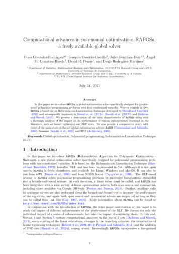
tree is a power of two. We tried other strategies, but we did not observe a significant impact on theresulting performance.Table 1b shows that the inclusion of a local solver has a huge impact on the performance of theRLT technique in both test sets. Performance improves in all dimensions, and specially so at closingthe gap, since the number of instances for which some bound is missing goes down from 144 to 0 inDS-TS and from 55 to 4 in MINLPLib-TS. Again, for this test set we have removed the 54 instancesin which the time limit is reached when generating the linear relaxation at the root node.We have run similar computational tests with different local NLP solvers and the results are quiterobust. Therefore, the specific choice of local solver does not seem to have a significant impact on thefinal performance of the RLT technique.4.3Different LP solversWe now check to what extent the chosen LP solver can make a difference in the performance of theRLT technique. To this end, we solve the instances in both test sets with three different solvers, twoopen source ones: CLP (Lougee-Heimer, 2003) and Glop (B. De Backer, 2015), and a commercial one:Gurobi (Gurobi Optimization, 2020).The results in Table 2 show that Gurobi’s performance is superior to both CLP and Glop. Onthe other hand, the two open source solvers are closed to one another. These is confirmed by theperformance profiles in Figure 7 in Appendix A.ClpGlopGurobiDS-TSsolved (128/180)gap av. timeav. gapmedian gapav. nodes1190163.150.040.03885.091190 2.39% 10.77% 3.54% 0.65%1270 24.46% 50.87% 61.95% 0.28%MINLPsolved (102/168)gap av. timeav. gapmedian gapav. nodes927178.942703.790.576463.11989 15.31% 99.96% 13.77% 31.97%996 37.55% 49.98% 3.15% 6.17%Table 2: Use of different linear solvers.4.4Parallelized RLTWe now move to an enhancement of a completely different nature. RAPOSa, as well as all branchand-bound algorithms, benefits from parallelization on multi-core processors. The way of exploringthe solutions tree in this type of strategy makes solving each node an independent operation, suitableto be distributed through processors in the same or different computational nodes. Hence, RAPOSa hasbeen parallelized, adapting the classic master-slave paradigm: a master processor guides the search inthe tree, containing a queue with pending-to-solve nodes (leaves), which will be sent to a set of workerprocessors. In this section, we present the computational results of our parallel version of RAPOSa,showing the obtained speedup as a function of the number of cores.More precisely, for each instance, RAPOSa was initially run in sequential mode (using one core) anda time limit of 10 minutes. Next, the parallel version was tested varying the numbers of cores andprompted to stop when each execution reached the same degree of convergence as in the non-parallelversion. Thus, the analysis focuses on the improvement on the time that the parallel version needs toreach the same result as the sequential one.Figure 1 shows the evolution of the speedup with the number of cores for DS-TS.6 In the x-axis werepresent the number of cores (master slaves) used by RAPOSa, while the y-axis shows the box plotof the speedup on the 180 DS-TS instances. The red line describes the ideal speedup: the number ofworkers. As can be seen, the scalability of the speedup obtained by the parallel version of RAPOSa is6 We do not include the results for MINLPLib-TS because the majority of the instances are either very easy or verydifficult, so the performance of the parallel version is harder to assess.7
, G H D O V S H H G X S 5 3 2 6 D * X U R E L 5 3 2 6 D * O R S 6 S H H G X S C R UesFigure 1: Speedup of the parallel version of RAPOSa in DS-TS.generally good, close to the ideal one when the number of cores is small (3 and 5) or with a reasonableperformance with a larger number of cores (9 and 17). Furthermore, the speedup does not seem todepend on the linear solver (Gurobi or Glop) used by RAPOSa.5Computational analysis of different enhancementsIn this section we present a series of additional enhancements of the basic implementation of theRLT technique and try to assess not only the individual impact of each of them, but also the aggregateimpact when different enhancements are combined. In order to do so, we define a baseline version ofRAPOSa that is used as the reference for the analysis, with the different enhancements being added tothis baseline. Given the results in the preceding section, this baseline configuration is set to use J-sets,Ipopt as the auxiliary local NLP solver,7 and Gurobi as the linear one. No parallelization is used.5.1Warm generation of J -setsWe start with an enhancement that is essentially about efficient coding, not really about theunderlying optimization algorithm.Along the branch and bound tree, the only difference between a problem and its father problem isthe upper or lower bound of a variable and the bound factors in which this variable appears. Becauseof this, it is reasonable to update only those bound-factor constraints that have changed instead ofregenerating all the bound-factor constraints of the child node.It is important to highlight that there are two running times involved in the process. One is therunning time used to generate the bound-factor constraints, which is higher in the case that RAPOSaregenerates all the bound-factor constraints. The other running time is the one used to identify thebound-factor constraints that change between the parent and the child node. This time is non-existentin the case that RAPOSa regenerates all the bound-factor constraints. As one could expect, the number0.00% in the last row of Table 1a reflects the fact that the warm gene
a freely available global solver Brais González-Rodríguez 1, Joaquín Ossorio-Castillo3, Julio González-Díaz1,3, Ángel M. González-Rueda2, David R. Penas1, and Diego Rodríguez-Martínez3 1Department of Statistics, Mathematical Analysis and Optimization, MODESTYA Research Group and IMAT, University of Santiago de Compostela.