WIXLIB

21. POLYNOMIALS IN ONE VARIABLEfrom the resultant (denoted Resx and discussed in Chapter 4) of the polynomialp(x) and its first derivative p0 (x) as follows:1· Resx (p(x), p0 (x)).adThis is an irreducible polynomial in the coefficients a0 , a1 , . . . , ad . It follows fromSylvester’s matrix formula for the resultant that the discriminant is a homogeneouspolynomial of degree 2d 2. Here is the discriminant of a quartic: f : a4 * x 4 a3 * x 3 a2 * x 2 a1 * x a0 : lprint(resultant(f,diff(f,x),x)/a4);discrx (p(x)) -192*a4 2*a0 2*a3*a1-6*a4*a0*a3 2*a1 2 144*a4*a0 2*a2*a3 2 144*a4 2*a0*a2*a1 2 18*a4*a3*a1 3*a2 a2 2*a3 2*a1 2-4*a2 3*a3 2*a0 256*a4 3*a0 3-27*a4 2*a1 4-128*a4 2*a0 2*a2 2-4*a3 3*a1 3 16*a4*a2 4*a0-4*a4*a2 3*a1 2-27*a3 4*a0 2-80*a4*a3*a1*a2 2*a0 18*a3 3*a1*a2*a0This sextic is the determinant of the following 7 7-matrix divided by a4: with(linalg): sylvester(f,diff(f,x),x);[ a4a3a2a1a000 ][][ 0a4a3a2a1a00 ][][ 00a4a3a2a1a0][][4 a43 a32 a2a1000 ][][ 04 a43 a32 a2a100 ][][ 004 a43 a32 a2a10 ][][ 0004 a43 a32 a2a1]Galois theory tells us that there is no general formula which expresses the rootsof p(x) in radicals if d 5. For specific instances with d not too big, say d 10, itis possible to compute the Galois group of p(x) over Q. Occasionally, one is luckyand the Galois group is solvable, in which case maple has a chance of finding thesolution of p(x) 0 in terms of radicals. f : x 6 3*x 5 6*x 4 7*x 3 5*x 2 2*x 1: galois(f);"6T11", {"[2 3]S(3)", "2 wr S(3)", "2S 4(6)"}, "-", 48,{"(2 4 6)(1 3 5)", "(1 5)(2 4)", "(3 6)"} solve(f,x)[1];1/12 (-6 (108 12 691/2 1/3)

1.2. NUMERICAL ROOT FINDING31/2 2/31/21/2 1/3 1/2 6 I (3 (108 12 69) 8 69 8 (108 12 69)) 72 )/1/2 1/3/ (108 12 69)/The number 48 is the order of the Galois group and its name is "6T11". Of course,the user now has to consult help(galois) in order to learn more.1.2. Numerical Root FindingIn symbolic computation, we frequently consider a polynomial problem assolved if it has been reduced to finding the roots of one polynomial in one variable. Naturally, the latter problem can still be very interesting and challengingfrom the perspective of numerical analysis, especially if d gets very large or if theai are given by floating point approximations. In the problems studied in thisbook, however, the ai are usually exact rational numbers with reasonably small numerators and denominators, and the degree d rarely exceeds 100. For numericallysolving univariate polynomials in this range, it has been the author’s experiencethat maple does reasonably well and matlab has no difficulty whatsoever. Digits : 6: f : x 200 - x 157 8 * x 101 - 23 * x 61 1: fsolve(f,x);.950624, 1.01796This polynomial has only two real roots. To list the complex roots, we say: fsolve(f,x,complex);-1.02820-.0686972 I, -1.02820 .0686972 I, -1.01767-.0190398 I,-1.01767 .0190398 I, -1.01745-.118366 I, -1.01745 .118366 I,-1.00698-.204423 I, -1.00698 .204423 I, -1.00028 - .160348 I,-1.00028 .160348 I, -.996734-.252681 I, -.996734 .252681 I,-.970912-.299748 I, -.970912 .299748 I, -.964269 - .336097 I,ETC.ETC.Our polynomial p(x) is represented in matlab as the row vector of its coefficients[ad ad 1 . . . a2 a1 a0 ]. For instance, the following two commands compute the threeroots of the dense cubic p(x) 31x3 23x2 19x 11. p [31 23 19 11]; roots(p)ans -0.0486 0.7402i-0.0486 - 0.7402i-0.6448Representing the sparse polynomial p(x) x200 x157 8x101 23x61 1 consideredabove requires introducing lots of zero coefficients: p [1 zeros(1,42) -1 zeros(1,55) 8 zeros(1,39) -23 zeros(1,60) 1] roots(p)ans

41. POLYNOMIALS IN ONE VARIABLE-1.0282 -1.0282 -1.0177 -1.0177 -1.0174 -1.0174 We note that convenient facilities are available for calling matlab inside of mapleand for calling maple inside of matlab. We encourage our readers to experimentwith the passage of data between these two programs.Some numerical methods for solving a univariate polynomial equation p(x) 0work by reducing this problem to computing the eigenvalues of the companion matrix of p(x), which is defined as follows. Let V denote the quotient of the polynomialring modulo the ideal hp(x)i generated by the polynomial p(x). The resulting quotient ring V Q[x]/hp(x)i is a d-dimensional Q-vector space. Multiplication bythe variable x defines a linear map from this vector space to itself.(1.2)Timesx : V V , f (x) 7 x · f (x).The companion matrix is the d d-matrix which represents the endomorphismTimesx with respect to the distinguished monomial basis {1, x, x2 , . . . , xd 1 } ofV . Explicitly, the companion matrix of p(x) looks like this: 0 0 ··· 0 a0 /ad 1 0 ··· 0 a1 /ad 0 1 ··· 0 a2 /ad (1.3)Timesx . . . . . . . .0 0 . . . 1 ad 1 /adProposition 1.2. The zeros of p(x) are the eigenvalues of the matrix Timesx .Proof. Suppose that f (x) is a polynomial in C[x] whose image in V C C[x]/hp(x)i is an eigenvector of (1.2) with eigenvalue λ. Then x · f (x) λ · f (x) inthe quotient ring, which means that (x λ) · f (x) is a multiple of p(x). Since f (x)is not a multiple of p(x), we conclude that λ is a root of p(x) as desired. Conversely,if µ is any root of p(x) then the polynomial f (x) p(x)/(x µ) represents aneigenvector of (1.2) with eigenvalue µ. Corollary 1.3. The following statements about p(x) Q[x] are equivalent: The polynomial p(x) is square-free, i.e., it has no multiple roots in C. The companion matrix Timesx is diagonalizable. The ideal hp(x)i is a radical ideal in Q[x].We note that the set of multiple roots of p(x) can be computed symbolicallyby forming the greatest common divisor of p(x) and its derivative:(1.4)q(x) gcd(p(x), p0 (x))Thus the three conditions in the Corollary are equivalent to q(x) 1.Every ideal in the univariate polynomial ring Q[x] is principal. Writing p(x) forthe ideal generator and computing q(x) from p(x) as in (1.4), we get the following

1.3. REAL ROOTS5general formula for computing the radical of any ideal in Q[x]: (1.5)Rad hp(x)i hp(x)/q(x)i1.3. Real RootsIn this section we describe symbolic methods for computing information aboutthe real roots of a univariate polynomial p(x). The Sturm sequence of p(x) is thefollowing sequence of polynomials of decreasing degree:p0 (x) : p(x), p1 (x) : p0 (x), pi (x) : rem(pi 2 (x), pi 1 (x)) for i 2.Thus pi (x) is the negative of the remainder on division of pi 2 (x) by pi 1 (x). Letpm (x) be the last non-zero polynomial in this sequence.Theorem 1.4. (Sturm’s Theorem) If a b in R and neither is a zero ofp(x) then the number of real zeros of p(x) in the interval [a, b] is the number of signchanges in the sequence p0 (a), p1 (a), p2 (a), . . . , pm (a) minus the number of signchanges in the sequence p0 (b), p1 (b), p2 (b), . . . , pm (b).We note that any zeros are ignored when counting the number of sign changesin a sequence of real numbers. For instance, a sequence of twelve numbers withsigns , , 0, , , , 0, , , 0, , 0 has three sign changes.If we wish to count all real roots of a polynomial p(x) then we can apply Sturm’sTheorem to a and b , which amounts to looking at the signs of theleading coefficients of the polynomials pi in the Sturm sequence. Using bisection,one gets a procedure for isolating the real roots by rational intervals. This methodis conveniently implemented in maple: p : x 11-20*x 10 99*x 9-247*x 8 210*x 7-99*x 2 247*x-210: sturm(p,x,-INFINITY, INFINITY);3 sturm(p,x,0,10);2 sturm(p,x,5,10);0 realroot(p,1/1000);1101 5511465 73314509 7255[[----, ---], [----, ---], [-----, ----]]1024 5121024 5121024512 fsolve(p);1.075787072, 1.431630905, 14.16961992Another important classical result on real roots is the following:Theorem 1.5. (Déscartes’s Rule of Signs) The number of positive real roots ofa polynomial is at most the number of sign changes in its coefficient sequence.For instance, the polynomial p(x) x200 x157 8x101 23x61 1, which wasfeatured in Section 1.2, has four sign changes in its coefficient sequence. Hence ithas at most four positive real roots. The true number is two.

61. POLYNOMIALS IN ONE VARIABLEIf we replace x by x in Descartes’s Rule then we get a bound on the numberof negative real roots. It is a basic fact that both bounds are tight when all rootsof p(x) are real. In general, we have the following corollary to Descartes’s Rule.Corollary 1.6. A polynomial with m terms has at most 2m 1 real zeros.The bound in this corollary is optimal as the following example shows:x·m 1Y(x2 j)j 1All 2m 1 zeros of this polynomial are real, and its expansion has m terms.1.4. Puiseux SeriesSuppose now that the coefficients ai of our given polynomial are not rationalnumbers but are rational functions ai (t) in another parameter t. Hence we wish todetermine the zeros of a polynomial in K[x] where K Q(t).(1.6)p(t; x) ad (t)xd ad 1 (t)xd 1 · · · a2 (t)x2 a1 (t)x a0 (t).The role of the ambient algebraically closed field containing K is now played bythe field C{{t}} of Puiseux series. The elements of C{{t}} are formal power seriesin t with coefficients in C and having rational exponents, subject to the condition that the set of exponents which appear is bounded below and has a commondenominator. Equivalently, [1C{{t}} C((t N )),N 1where C((y)) abbreviates the field of Laurent series in y with coefficients in C. Aclassical theorem in algebraic geometry states that C{{t}} is algebraically closed.For a modern treatment see [Eis95, Corollary 13.15].Theorem 1.7. (Puiseux’s Theorem) The polynomial p(t; x) has d roots,counting multiplicities, in the field of Puiseux series C{{t}}.The proof of Puiseux’s theorem is algorithmic, and, lucky for us, there is animplementation of this algorithm in maple. Here is how it works: with(algcurves): p : x 2 x - t 3;23p : x x - t puiseux(p,t 0,x,20);181512963{-42 t 14 t- 5 t 2 t - t t ,181512963 42 t- 14 t 5 t- 2 t t - t - 1 }We note that this implementation generally does not compute all Puiseux seriessolutions but only enough to generate the splitting field of p(t; x) over K. with(algcurves): q : x 2 t 4 * x - t: puiseux(q,t 0,x,20);29/215/241/2{- 1/128 t 1/8 t- 1/2 t t} S : solve(q,x): series(S[1],t,20);

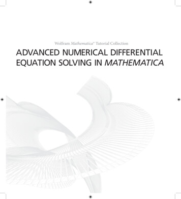
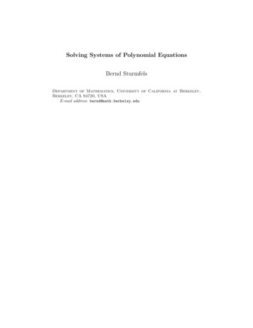
1.4. PUISEUX SERIES7Figure 1.1. The lower boundary of the Newton polygon1/2415/229/243/2t- 1/2 t 1/8 t- 1/128 t O(t) series(S[2],t,20);1/2415/229/243/2-t- 1/2 t - 1/8 t 1/128 t O(t)We shall explain how to compute the first term (lowest order in t) in each of thed Puiseux series solutions x(t) to our equation p(t; x) 0. Suppose that the ithcoefficient in (1.6) has the Laurent series expansion:ai (t)ci · tAi higher terms in t. Each Puiseux series looks likex(t)γ · tτ higher terms in t. We wish to characterize the possible pairs of numbers (τ, γ) in Q C which allowthe identity p(t; x(t)) 0 to hold. This is done by first finding the possible valuesof τ . We ignore all higher terms and consider the equation(1.7)cd · tAd dτ · · · c1 · tA1 τ c0 · tA0 · · · 0.This equation imposes the following piecewise-linear condition on τ :(1.8) min{Ad dτ, Ad 1 (d 1)τ, . . . , A2 2τ, A1 τ, A0 } is attained twice.The crucial condition (1.8) will reappear in Chapters 3 and 9. Throughout thisbook, the phrase “is attained twice” will always mean “is attained at least twice”.As an illustration consider the example p(t; x) x2 x t3 . For this polynomial,the condition (1.8) readsmin{ 0 2τ, 0 τ, 3 } is attained twice.That sentence means the following disjunction of linear inequality systems:2τ τ 3or 2τ 3 τor 3 τ 2τ.This disjunction is equivalent toτ 0orτ 3,which gives us the lowest terms in the two Puiseux series produced by maple.It is customary to phrase the procedure described above in terms of the Newtonpolygon of p(t; x). This polygon is the convex hull in R2 of the points (i, Ai ) fori 0, 1, . . . , d. The condition (1.8) is equivalent to saying that τ equals the slopeof an edge on the lower boundary of the Newton polygon. Figure 1.1 shows apicture of the Newton polygon of the equation p(t; x) x2 x t3 .

81. POLYNOMIALS IN ONE VARIABLE1.5. Hypergeometric SeriesThe method of Puiseux series can be extended to the case when the coefficientsai are rational functions in several variables t1 , . . . , tm . The case m 1 was discussed in the last section. An excellent reference on Puiseux series solutions forgeneral m is the work of John McDonald [McD95], [McD02].In this section we examine the generic case when all d 1 coefficients a0 , . . . , adin (1.1) are indeterminates. Each zero X of the polynomial in (1.1) is an algebraicfunction of d 1 variables, written X X(a0 , . . . , ad ). The following theorem dueto Karl Mayer [May37] characterizes these functions by the differential equationswhich they satisfy.Theorem 1.8. The roots of the general equation of degree d are a basis for thesolution space of the following system of linear partial differential equations: 2X ai aj(1.9)(1.10)Pdi 0 2X ak alwhenever Xiai a Xiandi j k l,Pd Xi 0 ai ai 0.The meaning of the phrase “are a basis for the solution space of” will beexplained at the end of this section. Let us first replace this phrase by “are solutionsof” and prove the resulting weaker version of the theorem.Proof. The two Euler equations (1.10) express the scaling invariance of theroots. They are obtained by applying the operator d/dt to the identitiesX(a0 , ta1 , t2 a2 , . . . , td 1 ad 1 , td ad )X(ta0 , ta1 , ta2 , . . . , tad 1 , tad )1t· X(a0 , a1 , a2 , . . . , ad 1 , ad ),X(a0 , a1 , a2 , . . . , ad 1 , ad ).Pdi 1To derive (1.9), we consider the first derivative f 0 (x) and the seci 1 iai xPdi 20ond derivative f 00 (x) i(i 1)ax.Notethatf(X) 60,sincea0 , . . . , adii 2Pdiare indeterminates. Differentiating the defining identityi 0 ai X(a0 , a1 , . . . , ad ) 0 with respect to aj , we get X j f 0 (X) ·(1.11) X aj 0.From this we derive f 0 (X) ai(1.12) f 00 (X)· X i iX i 1 .f 0 (X)We next differentiate X/ aj with respect to the indeterminate ai :(1.13) 2X Xj f 0 (X) j 0 X 0 0 X f (X) 2 jX j 1f (X) 1 . ai aj aif (X) ai aiUsing (1.11) and (1.12), we can rewrite (1.13) as follows: 2X ai aj f 00 (X)X i j f 0 (X) 3 (i j)X i j 1 f 0 (X) 2 .This expression depends only on the sum of indices i j. This proves (1.9). We check the validity of our differential system for the case d 2 and we notethat it characterizes the series expansions of the quadratic formula.

1.5. HYPERGEOMETRIC SERIES9 X : solve(a0 a1 * x a2 * x 2, x)[1];21/2-a1 (a1 - 4 a2 a0)X : 1/2 -----------------------a2 simplify(diff(diff(X,a0),a2) - diff(diff(X,a1),a1));0 simplify( a1*diff(X,a1) 2*a2*diff(X,a2) X );0 simplify(a0*diff(X,a0) a1*diff(X,a1) a2*diff(X,a2));0 series(X,a1,4);1/21/2(-a2 a0)1(-a2 a0)24----------- - 1/2 ---- a1 - 1/8 ----------- a1 O(a1 )a2a22a2 a0What do you get when you now type series(X,a0,4) or series(X,a2,4)?Writing series expansions for the solutions to the general equation of degree dhas a long tradition in mathematics. In 1757 Johann Lambert expressed the rootsof the trinomial equation xp x r as a Gauss hypergeometric function in the parameter r. Series expansions of more general algebraic functions were subsequentlygiven by Euler, Chebyshev and Eisenstein, among others. The widely known poster“Solving the Quintic with Mathematica” published by Wolfram Research in 1994gives a nice historical introduction to series solutions of the general equation ofdegree five:a5 x5 a4 x4 a3 x3 a2 x2 a1 x a0(1.14) 0.Mayer’s Theorem 1.8 can be used to write down all possible Puiseux series solutionsto the general quintic (1.14). There are 16 25 1 distinct expansions. For instance,here is one of the 16 expansions of the five roots: X2 aa12 aa01 ,X3 aa23 aa12 ,X1 aa10 , X4 aa34 aa23 ,X5 aa45 aa34 .Each bracket is a series having the monomial in the bracket as its first term: a0 a1 a1 a2 a2 a3 a3 a4 a4 a5 a0a1a1a2 a20 a2a31a21 a3a32 a2a3a3a4 a0 a5a23a2 a5a24a4a5 a31 a4a42 a30 a3a41a30 a22a51a40 a4a51a40 a2 a3a61 5a50 a5a61 a31 a33a52 a41 a5a52 5 2 a1 aa23 a5 a22 a4a33 a32 a5a43 2 a0 a21 a5a42 2 3a1 a4a23a23 a5a34 23a1 a25a34 3a2 a3 a25a44 a0 a35a44 4 ···a41 a3 a4a62a32 a24a53 ··· ···a1 a3 a35a54 ···

101. POLYNOMIALS IN ONE VARIABLEThe last bracket is just a single Laurent monomial. The other four bracketscan easily be written as an explicit sum over N4 . For instance, a0 a1X i,j,k,l 0 ai 1 ai( 1)2i 3j 4k 5l (2i 3j 4k 5l)! a0i 2j 3k 4l 1 ai2 aj3 ak4 al5·i ! j ! k ! l ! (i 2j 3k 4l 1)!a2i 3j 4k 5l 11Each coefficient appearing in one of these series is integral. Therefore these fiveformulas for the roots work in any characteristic. The situation is different for theother 15 series expansions of the roots of the quintic (1.14). For instance, considerthe expansions into positive powers in a1 , a2 , a3 , a4 . They are a1 a2 a3 a4 a1/512340 ξ ξ Xξ ξ · 1/5 · ξ3/5 2/52/5 3/51/5 4/55a5a5a0 a5a0 a5a0 a5where ξ runs over the five complex roots of the equation ξ 5 1, and a1/5 01/5a5 a1 3/5 2/5a0 a5 a2 2/5 3/5a0 a5 a3 1/5 4/5a0 a51/5 a01/5a5 a1 a4125 a4/5 a6/505 a2 a3125 a4/5 a6/505 a21 a32125 a9/5 a6/505 a2 a243125 a4/5 a11/505 ···a13/5 2/5a5 a2315 a3/5 a7/505 2 a2 a45 a3/5 a7/505 a3 a24725 a3/5 a12/505 6 a1 a2 a325 a8/5 a7/505 ··· a22/5 3/5a0 a5 a2115 a7/5 a3/505 3 a3 a45 a2/5 a8/505 6 a1 a2 a425 a7/5 a8/505 a1 a23325 a7/5 a8/505 ··· a31/5 4/5a0 a5 1 a1 a25 a6/5 a4/505 a2425 a1/5 a9/505 a31125 a11/5 a4/505 a0 4 a1 a3 a425 a6/5 a9/505 ···Each of these four series can be expressed as an explicit sum over the lattice points ina 4-dimensional polyhedron. The general formula can be found in [Stu00, Theorem3.2]. That reference gives all 2d 1 distinct Puiseux series expansions of the solutionof the general equation of degree d.The system (1.9)-(1.10) is a special case of the hypergeometric differential equations discussed in [SST99]. More precisely, it is the Gel’fand-Kapranov-Zelevinskysystem with parameters 1associated with the integer matrix0 0 1

The purpose of this chapter is to provide some basic tools for this problem. We shall consider the problem of how to compute and how to represent the zeros of a general polynomial of degree din one variable x: (1.1) p(x) a dxd a d 1xd 1 ··· a 2x2 a 1x a 0. 1.1. The Fundamental Theorem of Algebra We begin by assuming that the .