Transcription
ECE 645: Estimation TheorySpring 2015Instructor: Prof. Stanley H. ChanLecture Note 1: Bayesian Decision Theory(LaTeX prepared by Stylianos Chatzidakis)March 31, 2015This lecture note is based on ECE 645(Spring 2015) by Prof. Stanley H. Chan in the School ofElectrical and Computer Engineering at Purdue University.1IntroductionClassification appears in many disciplines for pattern recognition and detection methods. In thislecture we introduce the Bayesian decision theory, which is based on the existence of prior distributions of the parameters.1.1Bayesian Detection FrameworkBefore we discuss the details of the Bayesian detection, let us take a quick tour about the overallframework to detect (or classify) an object in practice. In the Bayesian setting, we model observations as random samples drawn from some probability distributions. The classification processusually involves extracting features from the observations, and a decision rule that satisfies certainoptimality criterion. See Figure 1.MeasurementFeature ExtractionClassifierClassificationFigure 1: Block diagram of a classifierWhen the distributions of the random samples are not known (which is true in most real-worldapplications), we might need an estimation algorithm to first determine the parameters of thedistributions, e.g., mean and standard deviation. A decision rule can then designed based on theseestimated parameters. To verify the efficiency of the classifier, testing data are used to calculatethe error rate or false alarm rate. In most cases, a classifier with small false alarm rate is sought.This process is shown in Figure 2.MeasurementFeature ExtractionClassifierEstimation AlgorithmClassificationTraining DataFigure 2: classifierIn practice, of course, all the above building blocks have to be taken into account. However, tohelp us understand the important ideas of the detection theory, we will focus on the design of the
classifiers in this course. Interested readers can consult standard textbooks on pattern recognitionsfor detailed discussions on these practical issues.1.2Objectives and OrganizationsWe begin this lecture note with a brief review of probability. We assume that readers are familiarwith introductory probability theory (e.g., ECE 600). After reviewing probability theory, we willdiscuss the general Bayes’ decision rule. Then, we will discuss three special cases of the generalBayes’ decision rule: Maximum-a-posteriori (MAP) decision, Binary hypothesis testing, and M-aryhypothesis testing.22.1Review of ProbabilityProbability SpaceAny random experiment can be defined using the probability space (S, F, P) where S is the samplespace, F is the event space, and P is the probability mapping. The sample space S is a non-emptyset containing all outcomes of the experiments. The event space F is a collection of subsets of Sto which probabilities are assigned. The event space F must be a non-empty set that satisfies theproperties of a σ-field. The probability mapping is a set function that assigns a real number toevery set:P:F R(1)and must satisfy the following three probability P(A) 0, for all A FP(S) 1P(A B) P(A) P(B) if A B .Conditional ProbabilityIn many situations we would want to know the probability of an event A occurring given thatanother event B has occurred. In this case, the probability of an event A given that another eventB has occured is called conditional probability. The condition probability of A given B is definedas:P(A B) P(A B)P(B)(2)assuming P(B) 0.Example 1.Consider rolling a die. The probability of event A 6 is equal to 1/6. However, if someoneprovides additional information, let’s say that the event B roll of a die was bigger than 4, thenthe probability of A given B is:P(A B) P(A B)1/6 1/3.P(B)3/62
A simple calculation of conditional probability allows us to write:P(A B) P(A B)P(B)(3)P(B A) P(B A)P(A)(4)andthen equating the left and right hand sides we can derive the Bayes’ Theorem:Theorem 1. Bayes’ TheoremFor any events A and B such that P(B) 0,P(B A)P (A).P(B)P(A B) (5)The Bayes’ theorem can be generalized to yield the following result.Theorem 2. Law of Total ProbabilityIf A1 , A2 , . . . , An is a partition of the sample space and B is an event in the event space, thenP(B) nXP(B Ai )P(Ai )(6)i 1The law of total probability suggests that for any event B, we can decompose B into a sum ofn disjoint subsets Ai . Moreover, applying the total probability law to Bayes theorem yieldsP(B A)P (A)P(A B) Pni 1 P(B Ai )P(Ai )(7)for A, B F, P(A) 0 and P(B) 0.2.3Random VariablesA random variable is a real function from the sample space to the real numbers:X :S R(8)A random variable can be discrete or continuous. For the discrete case, the probability massfunction is defined aspX (x) P(ω S : X(ω) x)(9)For the continuous case, the cumulative distribution function is defined asFX (x) P(ω S : X(ω) x)(10)When the cumulative distribution function is differentiable, we can define the probability densityfunction asdfX (x) FX (x).(11)dx3
2.4ExpectationsThe expectation of a random variable described by a probability mass function or a probabilitydensity function is(PxpX (x),if X is discrete,E[X] R (12)if X is continuous. xfX (x)dx,The conditional expectation isE[X Y y] Z xfX Y (x y)dx(13)The variance is defined as:Var[X] E[(X E[X])2 ] E[X 2 ] E[X]2 .(14)A very useful result of the expectation is the total expectation formula, also known as theiterated expectation.Theorem 3. Total ExpectationE[X] EY [EX Y [X Y y]](15)Proof.Z Z xfX (x)dx xfXY (x, y)dxdy Z Z xfX Y (x y)dydx Z Z fY (y)xfX Y (x y)dx Z E[X Y y]fY (y)dy EY [EX Y [X Y y]]. E[X] Z 2.5Gaussian DistributionFinally we review the Gaussian distribution. A single variable Gaussian distribution is defined as11fX (x) e 2πσ 2 x µσ 2,(16)where µ is the mean and σ 2 is the variance. We writeX N (µ, σ 2 )to denote a random variable X drawn from a Gaussian distribution.4(17)
For multivariate Gaussian, the distribution is 11T 1exp Σ(x µ),fX (x) (x µ)2(2π)d/2 Σ 1/2(18)where X [X1 , X2 , · · · , Xd ]T is a d-dimensional vector, µ [µ1 , µ2 , · · · , µd ]T is the mean vector,and Var(X1 )· · · Cov(X1 , Xd ) .(19)Σ E[(X µ)(X µ)T ] .Cov(X1 , Xd ) · · ·Var(Xd )is the covariance matrix.If Cov(Xi , Xj ) 0 then Xi and Xj are said to be uncorrelated. If Cov(Xi , Xj ) 0 thenXi and Xj are said to be positively correlated. However, it should be clarified that uncorrelateddoes not imply independent, because Cov(X, Y ) 0 only implies E[XY ] E[X]E[Y ] but notfX,Y (x, y) fX (x)fY (y). The converse is true however. That is, if X and Y are independent, thenCov(X, Y ) 0. Here is a counter example by C. Shalizi.Example 2.Let X Uniform( 1, 1), and let Y X . Then,E[XY X 0] E[XY X 0] Z1x2 dx 1/30Z0 1x2 dx 1/3.Thus, by Law of Total Expectation we have E[XY ] 0. However, X and Y are clearly dependent.3Bayesian Decision TheoryIn Bayes’s detection theory, we are interested in computing the posterior distribution fΘ X (θ x).Using Bayes’ theorem, it is easy to show that the posterior distribution fΘ X (θ x) can be computedvia the conditional distribution fX Θ (x θ) and the prior distribution fΘ (θ). The prior distributionfΘ (θ) represents the prior knowledge we may have for the distribution of the θ parameter beforewe obtain additional information for our dataset. In other words, Bayes’ detection theory utilizesprior knowledge in the decision.Bayes’ theorem can be used for discrete or continuous random variables. For discrete randomvariables it takes the form:pY Θ (y θ)pΘ (θ)pΘ Y (θ y) ,(20)pY (y)where p represents the probability mass function. For continuous random variables:fΘ Y (θ y) fY Θ (y θ)fΘ (θ),fY (y)where f is the probability density function.5(21)
3.1NotationsTo facilitate the subsequent discussion, we introduce the following notations.1. Parameter Θ. We assume that Θ is a random variable with realization Θ θ. The domainof θ is defined as Λ. For detection, we assume that Λ is a collection of M states, i.e.,defΛ {0, 1, ., M 1}.2. Prior distributions π0 , π1 , . . . , πM 1 , where πj P(Θ j). Note that the sum of all πj shouldbe 1:M 1Xπj 1.(22)j 03. Conditional distribution of observing Y y given that Θ j:deffj (y) P(Y y Hj ),(23)where Hj denotes the hypothesis that Θ j.4. Posterior distributions of having Θ j given the observation Y y:defπj (y) P(Hj Y y).(24)By Bayes’ theorem, we can show thatP(Hj Y y) and soP(Y y Hj )p(Hj ),P(Y y)fj (y)πjπj (y) P.j fj (y)πj(25)(26)5. Decision rule δ : Γ Λ. The decision rule is a function that takes an input y Γ and sendsy to a value δ(y) Λ.6. Cost function C(i, j) or Cij . In detection or classification of objects, every decision is accompanied by a cost. If, for example, there is a flying object or a disease and we are not ableto detect, then there is cost with this decision. That is, if we decide that there is no signalbut instead there is signal, then we call this a miss. In the case were there is nothing presentbut we decide that there is, then we have a false alarm. Sometimes the cost is very small orsignificant depending on the situation. For example, it is preferable to have false alarm thana miss in the case of disease detection. The cost associated with each decision is described bythe cost function. Here, we use Cij to describe the cost of choosing Hi when Hj holds. For abinary hypothesis, the cost function can be represented by a table:H0C00C10δ(y) 0δ(y) 1H1C01C11For example, C01 is the cost associated with selecting H0 when H1 was the true value, i.e.,the cost of having a miss. Similarly, C10 is the cost of having a false alarm. C00 and C11 arethe cost of having the correct detection.6
3.2Bayesian RiskThe goal of Bayesian detection is to minimize the risk, defined asR(δ) EY Θ [C(δ(Y ), Θ)].(27)In other words, the optimal decision rule isδ(y) argmin R(δ).(28)δMinimizing the risk defined as the expectation of the cost function is analytically very difficult asit involves the minimization of the double integral. To solve this problem we observe the followingresult:Proposition 1.δ(y) argmin EY Θ [C(δ(Y ), Θ)] argminiδM 1XC(i, j)πj (y).(29)j 0To prove the above proposition we need to make use of the total expectation, and in particularthe following lemma:Lemma 1.EY Θ [C(δ(Y ), Θ)] EY [EΘ Y [C(δ(Y ), Θ) Y y]].(30)Proof.By definition of EY Θ [C(δ(Y ), Θ)], we haveEY Θ [C(δ(Y ), Θ)] ZZC(δ(y), θ)fY Θ (y, θ)dydθ.Since fY Θ (y, θ) fΘ Y (θ y)fY (y) by Bayes’ theorem, we haveZZEY Θ [C(δ(Y ), Θ)] C(δ(y), θ)fΘ Y (θ y)fY (y)dθdy.Switching the order of integration yieldsZZZZC(δ(y), θ)fΘ Y (θ y)fY (y)dθdy fY (y) C(δ(y), θ)fΘ Y (θ y)dθdy,in which we see that the inner integration is EΘ Y [C(δ(Y ), θ) Y y]. Therefore,ZZZfY (y) C(δ(y), θ)fΘ Y (θ y)dθdy fY (y)EΘ Y [C(δ(Y ), θ) Y y]dy EY [EΘ Y [C(δ(Y ), Θ) Y y]]. Using the Lemma we can prove the proposition.7
Proof.By Lemma, we have thatZargmin EY Θ [C(δ(Y ), Θ)] argminδδEΘ Y [C(δ(Y ), Θ) Y y]fY (y)dy.Since fY (y) is non-negative, the minimizer of the integral is the same as the minimizer of the innerexpectation. Therefore, we haveargmin EY Θ [C(δ(Y ), Θ)] argmin EΘ Y [C(δ(Y ), Θ) Y y].δδExpressing out the definition of the conditional expectation, we haveδ(y) argminiM 1XC(i, j)πj (y).j 0 We remark that δ(y) is a function of y. That is, for a different observation y, the decision valueδ(y) is different. To denote that this the Bayesian decision rule, we put a subscript δB (y).3.3Maximum-A-Posteriori ruleWe now consider a special case where the cost function is uniform, defined as(1, i 6 j,C(i, j) 0, i j.(31)In this case, the decision rule becomesδB (y) argmini argminiM 1XC(i, j)πj (y)j 0M 1Xπj (y)j 0 argmin (1 πj (y))i argmax πi (y).iTherefore, for uniform cost, the risk is minimized by maximizing the posterior distribution. Thuswe call the resulting decision rule as the Maximum-A-Posteriori (MAP) rule.An important property of the MAP rule is that is minimizes the probability of error.Definition 1.The probability of error is defined asPerror P(Θ 6 δ(Y )).8(32)
Proposition 2.For any decision rule δ, and for a uniform cost,Perror R(δ).Proof.First of all, we note by the law of total probability thatZ P(Θ 6 δ(Y ) Y y)fY (y)dy.Perror P(Θ 6 δ(Y )) The conditional probability inside the integral can be written as:P(Θ 6 δ(Y ) Y y) 1 P(Θ δ(Y ) Y y) M 1XP(Θ j Y y).j 0By using the uniform cost, we haveM 1XP(Θ δ(Y ) Y y) j 0M 1XC(δ(y), j)P(Θ δ(Y ) Y y)j 0 EΘ Y [C(δ(Y ), Θ), Θ Y ].Therefore the probability of error becomes:Z ZPerror P(Θ 6 δ(Y ) Y y)fY (y)dy EΘ Y [C(δ(Y ), Θ), Θ Y ]fY (y)dy,which is equal to the expectation of the cost which is the definition of the risk. Therefore,Perror EY [C(δ(Y ), Θ] R(δ). The result of this proposition says that since the probability of error is equal to the risk for thecase of a uniform cost function, and since the Bayes’ decision rule minimizes the risk, the Bayes’decision rule should also minimize the probability of error.3.4Binary Hypothesis TestingWe now discuss the binary hypothesis testing problem. To begin with, let us consider the generalcost function. Denoting C00 , C01 , C10 , C11 as the cost and π0 , π1 as the prior, we can write Bayesiandecision rule asδB (y) argminiM 1Xj 09Cij πj (y).
Since there are only two possible choices of decisions (because it is a binary decision problem), wehave0C00 π0 (y) C01 π1 (y) HH1 C10 π0 (y) C11 π1 (y).With some simple calculations we can show that0C00 π0 (y) C01 π1 (y) HH1 C10 π0 (y) C11 π1 (y)0 π1 (y)(C01 C11 ) HH1 π0 (y)(C10 C00 )π1 (y)0 C10 C00 H π0 (y)H1 C01 C11 ,where the last inequality follows because C00 C10 and C11 C01 . Since πj (y) havePfj (y)πj ,j fj (y)πjwef1 (y) H0 (C00 C10 )π0. f0 (y) H1 (C11 C01 )π1If we definedefL(y) anddefη then the decision rule becomesf1 (y),f0 (y)(C00 C10 )π0,(C11 C01 )π10L(y) HH1 η.The function L(y) is called the likelihood ratio and the above decision rule the likelihood rationtest (LRT).Example 3.Let two sample data drawn from two classes. The classes are described by two Gaussian distributions having equal variance but different means:H0 :Y N (0, σ 2 )H1 :Y N (µ, σ 2 )To determine the Bayes’ decision rule, we first compute the likelihood ratio 1 y µ 2e 2 ( σ )2yµ µ2L(y) exp .1 y 22σ 2e 2 ( σ )By taking log on both sides, we have0ln L(y) HH1 ln(C00 C10 )π0 def ln η.(C11 C01 )π1With some calculations we can show that this is equivalent to0y HH1σ 2 ln η µ .µ2Thus, if the observed value y is larger that the right hand side of the above equation then mustchoose class i 1. If not, we must choose class i 0. Figure 3 illustrates an numerical examplefor the 1D and the 2D case.10
2.701.2Class HClass HClass H01Class H2.65011.0Decision boundary2.602.55Y valuesarbitrary scale0.80.62.502.450.42.40Decision .77.8X valuesX valuesFigure 3: Decision boundaries for a binary hypothesis testing problem of 1D and 2D Gaussian.The above general Bayes decision rule can be simplified when we assume a uniform cost. Inthis case, we havef1 (y) H0 π0 ,f0 (y) H1 π1which is equivalent to0π1 (y) HH1 π0 (y).Therefore, we will claim H0 if π0 (y) π1 (y) and vice versa. Or equivalently, we haveδ(y) argmax πi (y).iSince πi (y) is the posterior probability, we can the resulting decision rule as the maximum-aposteriori decision.Example 4.Consider Example 3 with uniform cost. Then, the MAP decision rule is (with η 1)y 3.5µ.2M-ary Hypothesis TestingWe can generalize the above binary hypothesis testing problem to a M -ary hypothesis testingproblem. In M-ary hypothesis testing, there are M hypotheses or classes which we wish to assignour observations. The Bayesian decision rule is based again on minimizing the risk similarly to thebinary case:M 1XδB (y) argminC(i, j)πj (y).(33)ij 011
By Bayes’ theorem, we haveδB (y) argminiM 1XC(i, j)j 0πj fj (y).f (y)Now, we can divide the posterior distribution by the posterior of H0 without affecting the minimizerof the optimizaiton:δB (y) argmini argminiπj fj (y)f (y)C(i, j) π f (y)0 0j 0f (y)M 1XM 1XC(i, j)j 0,πj fj (y).π0 f0 (y)By definingdefLj (y) M 1Xfj (y)πj, and hi (y) C(i, j) Lj (y),f0 (y)π0j 0we can show thatδB (y) argmin hi (y).iTherefore, our goal is to select hypothesis H0 if h0 h1 and h0 h2 and h0 h3 up toh0 hM 1 . To visualize this, let’s consider three hypotheses described by three 1-d Gaussiandistributions (Figure 4). In this case, there can be no single boundary as in the binary hypothesistesting, instead the observed value has to be compared with all individual hypotheses to reach aconclusion.TO DO: Add an example to example M-ary hypothesis testing.4Numerical ExampleIn this example, we generate data from a random number generator. Our goal is to use Bayes’decision rule to classify the data into 2 classes. The m-file is provided in the appendix. Two setsof experiments were performed. The first one was based on equal priors for class 1 and class 2,π1 π2 0.5. 1000 samples were drawn. The probability density functions were assumed to beGaussian to represent the two classes but they differed in mean value. Two typical probabilitydensity distributions that were used and the sampled data are shown in Figure 5a. For differentpriors π1 0.9 and π2 0.1 the probability density distributions that were used and the sampleddata are shown in Figure 5b. It can be seen that the sampled data for the second pdf are morescarce. However, the decision boundary can be easily drawn. Finally, two pdfs with differentstandard deviations is shown in Figure 6. In this case, there is significant overlap between the twodistributions and the decision boundary is more complicated than before.For simplicity, let’s start the classification example with equal standard deviations for bothGaussians distributions, i.e., σ1 σ2 2.0. For class 1, the average value was selected to bem1 1.0 and was kept constant. For class 2, the average value m2 varied from 4.0 to 20.0 with a stepof 2. That is m2 4, 6, 8, 10, 12, 14, 16, 18, 20 and therefore m2 m1 3, 5, 7, 9, 8, 11, 13, 15, 17, 19.This experiment was performed 10 times and the number of misclassifications was measured asshown in the following Figure 7a. The priors were different in this case, π1 0.2 and π2 0.8.12
8Class HClass H7Class H210arbitrary scale65432106.66.87.07.27.47.67.88.0X valuesFigure 4: M 3 hypothesesIt appears that increasing the distance between the distributions, the error is reduced and fromapproximately 90 decreases to 0 for m2 m1 12. Therefore, for completely separated classes themisclassifications are almost zero, as expected.The second experiment considers equal priors, π1 0.5 and π2 0.5. The results are showngraphically in Figure 7b. In this case, the number of misclassifications is larger and approachesapproximately 250 for mean different less than 4.Overall, it was shown that for well separated classes the error of classification is very smalland tends asymptotically to zero as the separation increases. On the contrary, for poor separationbetween the two classes the error was large and was approaching the priors. Finally, it is observedthat when the priors and the probability density distributions are known, Bayes rule is an efficientand simple tool to provide classification decisions in an optimal way.5ReferencesC.M. Bishop, 2006. Pattern Recognition and Machine Learning, SpringerR. O. Duda, P. E. Hart, and D. G. Stork. 2000, Pattern Classification (2nd Edition). WileyInterscience.K. Fukunaga, 1990. Introduction to Statistical Pattern Recognition (2nd Edition). AcademicPress Prof., Inc., San Diego, CA, USA.A. Papoulis and S. U. Pillai, Probability, 2001. Random Variables and Stochastic Processes,McGraw-Hill.13
0.30.3Data sampled from pdf with 1.0Data sampled from pdf with 1.0Data sampled from pdf with 8.0Data sampled from pdf with 8.0PDF withPDF with 1.0PDF with 1.0 8.0PDF with 8.0P P 0.51P 0.9, P -20246810121416-6Sampled data-4-20246810121416Sampled data(a) Equal priors(b) Different priorsFigure 5: Gaussian distributions and sampled data6AppendixMatlab %%%%%%%%%%%%%%%%%%%%%% This m-file calculates the number of misclassifications of a% classification algorithm using Bayes rule. There are 100 data% that belong to 2 different classes drawn from a random number generator.% Bayes rule is used to classify the data. The experiment is repeated% 10 times for each m2-m1 0,2,4,6,8 and priors P1 P2 0.5 (i.e., 50 experiments total)% and 10 times for each m2-m1 0,2,4,6,8 and priors P1 0.2 and P2 0.8. m1% and m2 are the mean values of the Gaussian distribution. Sigma1 and% sigma2 are the standard deviations of the Gaussian %%%%%%%%%%%%%%%%%%%%%%%%%%%%%%clc;clear all;P1 0.5;% prior for class 1P2 0.5;% prior for class 2m1 1.0;% mean for normal distribution class 1mu111 1.0071;su111 3.9004;sigma1 2.0; % standard deviation for normal distribution class 1m2 16.0;% mean for normal distribution class 2sigma2 2.0; % standard deviation for normal distribution class 2mu222 2.983;su222 3.953;N(1) 1000;for n 1:1for k 1:1% increase number of datafor j 1:10% perform experiment 10 times14
0.3Data sampled from pdf with 1.0Data sampled from pdf with 8.0PDF with 1.0PDF with 8.0P 0.9, P 0.112Probability0.20.10.0-8-404812162024Sampled dataFigure 6: Gaussian distributions with different standard deviations and priorsfor i 1:N(k)% 100 randomly selected datar rand;if r P2c(i) 1;% class 1r1(i) m1 sigma1*randn;r2(i) r1(i);r3(i) 0;elsec(i) 2;% class 2r1(i) m2 sigma2*randn;r2(i) 0;r3(i) r1(i);endg1(i) pdf('Normal',r1(i),m1,sigma1)*P1;%calculate probabilityg2(i) pdf('Normal',r1(i),m2,sigma2)*P2;% calculate probabilityg(i) g1(i)-g2(i);% take the differenceif g(i) 0% if g 0 then class 1y(i) 1;elsey(i) 2;endm(i) abs(c(i)-y(i));% if c-y 0 then correct classificationsendA [c',y',m'];mi(k,j) nnz(m'); % returns the number nonzero elements of matrix kendmu(k) mean(mi(k,j));%calculate average of misclassifications for 10 experimentssd(k) std(mi(k,j));% standard deviation of misclassifications for 10 experimentsmi(k,j);15
120300P 0.9, P 0.1P 0.5, P ns1604020021501005002468101214161820022Mean difference02468101214Mean difference(a) Different priors(b) Equal priorsFigure 7: Misclassifications for equal and different priorsN(k 1) N(k) 100;endDm m2-m1;% difference of meansfigure(3)hold onplot(Dm,mu(k),'o')figure(4)hold onplot(Dm,mi(k,:),'o')m2 m2 0;endpdf2 pdf('Normal',r2,m1,sigma1);pdf3 2022
The sample space S is a non-empty set containing all outcomes of the experiments. The event space F is a collection of subsets of S to which probabilities are assigned. The event space F must be a non-empty set that satisfies the . Consider rolling a die. The probability of event A 6 is equal to 1/6. However, if someone provides additional .