Transcription
Matlab Tutorial : Root LocusECE 3510Heather Malko
Table of Context 1.0Introduction 2.0Root Locus Design 3.0SISO Root Locus 4.0GUI for ControlsThe University of Utah
1.0 Introduction A root loci plot is simply a plot of the s zero values andthe s poles on a graph with real and imaginaryordinates. The root locus is a curve of the location of the poles of atransfer function as some parameter (generally the gainK) is varied. The locus of the roots of the characteristic equation ofthe closed loop system as the gain varies from zero toinfinity gives the name of the method. This method is very powerful graphical technique forinvestigating the effects of the variation of a systemparameter on the locations of the closed loop poles.The University of Utah
1.0 Introduction General rules for constructing the root locus exist and ifthe designer follows them, sketching of the root locibecomes a simple matter. Root loci are completed to select the best parametervalue for stability. A normal interpretation of improving stability is when thereal part of a pole is further left of the imaginary axis.The University of Utah
1.0 Introduction Matlab and Root Locus:MATLAB Control System Toolbox containstwo Root Locus design GUI, sisotool andrltool. These are two interactive design toolsof SISO.The University of Utah
1.0 Introduction Matlab’s Useful Commands : b cmds.html ntro.html http://users.ece.gatech.edu/ bonnie/book/TUTORIAL/tut 3.htmlThe University of Utah
2.0 Root Locus Tutorial # 1 Key Matlab commands used in this tutorial:cloop, rlocfind, rlocus, sgrid, step Matlab commands from the control systemtoolbox are highlighted in red.The University of Utah
2.0 Root Locus Design The root locus of an (open-loop) transfer function H(s) isa plot of the locations (locus) of all possible closed looppoles with proportional gain k and unity feedback:The University of Utah
2.0 Root Locus Design The closed-loop transfer function is: and thus the poles of the closed loop system arevalues of s such that 1 K H(s) 0.If H(s) b(s)/a(s), then this equation has the form:Let n order of a(s) and m order of b(s) [theorder of a polynomial is the highest power of s thatappears in it].The University of Utah
2.0 Root Locus Design Consider all positive values of k.In the limit as k - 0, the poles of the closed-loop systemare a(s) 0 or the poles of H(s).In the limit as k - infinity, the poles of the closed-loopsystem are b(s) 0 or the zeros of H(s).No matter what we pick k to be, the closed-loopsystem must always have n poles, where n is thenumber of poles of H(s). The root locus must have nbranches, each branch starts at a pole of H(s) andgoes to a zero of H(s).The University of Utah
2.0 Root Locus Design Consider an open loop system which has a transferfunction ofnum [1 7];den conv(conv([1 0],[1 5]),conv([1 15],[1 20]));rlocus(num,den)axis([-22 3 -15 15])The University of Utah
2.0 Root Locus DesignRoot Locus1510Imaginary Axis50-5-10-15-20-15-10Real A xisThe University of Utah-50
2.0 K from the root locus The plot above shows all possible closed-loop polelocations for a pure proportional controller.So use the command sgrid(Zeta,Wn) to plot lines ofconstant damping ratio and natural frequency.Its two arguments are the damping ratio (Zeta) andnatural frequency (Wn) [these may be vectors if youwant to look at a range of acceptable values]. In theproblem, an overshoot less than 5% (which means adamping ratio Zeta of greater than 0.7) and a rise timeof 1 second (which means a natural frequency Wngreater than 1.8).The University of Utah
2.0 K from the root locus zeta 0.7; Wn 1.8; sgrid(zeta, Wn)Root Locus1510Imaginary Axis50.71.800.7-5-10-15-20-15-10Real AxisThe University of Utah-50
2.0 K from the root locus The plot above shows all possible closed-loop polelocations for a pure proportional controller.So use the command sgrid(Zeta,Wn) to plot lines ofconstant damping ratio and natural frequency.Its two arguments are the damping ratio (Zeta) andnatural frequency (Wn) [these may be vectors if youwant to look at a range of acceptable values]. In theproblem, an overshoot less than 5% (which means adamping ratio Zeta of greater than 0.7) and a rise timeof 1 second (which means a natural frequency Wngreater than 1.8).The University of Utah
2.0 K from the root locus [kd,poles] rlocfind(num,den)Root Locus1510Imaginary Axis50.71.800.7-5-10-15-20The University of Utah-15-10Real Axis-50
2.0 K from the root locus [kd,poles] rlocfind(num,den)Select a point in the graphics windowselected point -2.6576 0.0466ikd 306.9457poles 1) -21.81802) -12.57943) -2.93734) -2.6652The University of Utah
2.0 Closed-loop response In order to find the step response, one needs to knowthe closed-loop transfer function. [numCL, denCL] cloop((kd)*num, den)The two arguments to the function cloop are thenumerator and denominator of the open-loop system.You need to include the proportional gain that you havechosen. Unity feedback is assumed.If you have a non-unity feedback situation, look at thehelp file for the Matlab function feedback, which can findthe closed-loop transfer function with a gain in thefeedback loop.The University of Utah
2.0 Closed-loop response [numCL, denCL] cloop((kd)*num, den)numCL 1.0e 003 * 0000.3069 2.1486denCL 1.0e 003 * 0.0010 0.04000.4750 1.8069 2.1486 step(numCL,denCL)The University of Utah
2.0 Closed-loop responseStep 11.5Time (sec)The University of Utah22.5
2.0 Root Locus DesignThe University of Utah
2.0 Root Locus Design cus/rlocus.html urses/414/lab1/matlabcommands.pdfThe University of Utah
3.0 SICO Root Locus Design Design ConstraintsWhen designing compensators, it is common to havedesign specifications that call for specific settling times,damping ratios, and other characteristics.The SISO Design Tool provides design constraints thatcan help make the task of meeting design specificationseasier. The New Constraint window, which allows youto create design constraints, automatically changes toreflect which constraints are available for the view inwhich you are working.The University of Utah
3.0 SICO Root Locus Design Design ConstraintsSelect Design Constraints and then New to open theNew Constraint window, which is shown below.The University of Utah
3.0 SICO Root Locus Design Design Constraints for the Root Locus For the root locus, you have the following constrainttypes:Settling TimePercent OvershootDamping RatioNatural Frequency The University of Utah
3.0 SICO Root Locus Design Settling Time. If you specify a settling time in thecontinuous-time root locus, a vertical line appears onthe root locus plot at the pole locations associated withthe value provided (using a first-order approximation). Inthe discrete-time case, the constraint is a curved line.Percent Overshoot. Specifying percent overshoot inthe continuous-time root locus causes two rays, startingat the root locus origin, to appear. These rays are thelocus of poles associated with the percent value (usinga second-order approximation). In the discrete-timecase, In the discrete-time case, the constraint appearsas two curves originating at (1,0) and meeting on thereal axis in the left-hand plane.The University of Utah
3.0 SICO Root Locus Design Damping Ratio. Specifying a damping ratio in thecontinuous-time root locus causes two rays, starting atthe root locus origin, to appear. These rays are thelocus of poles associated with the damping ratio. In thediscrete-time case, the constraint appears as curvedlines originating at (1,0) and meeting on the real axis inthe left-hand plane. Natural Frequency. If you specify a natural frequency,a semicircle centered around the root locus originappears. The radius equals the natural frequency.The University of Utah
3.0 SICO Root Locus Design load ltiexamplessisotool(sys dc)The University of Utah
3.0 SICO Root Locus Design The two rays centered at (0,0) represent the dampingratio constraint. The dark edge is the region boundary,and the shaded area outlines the exclusion region. Thisfigure explains what this means for this constraint. use this design constraint to ensure that the closed-looppoles, represented by the red squares, have someminimum damping. Try adjusting the gain until thedamping ratio of the closed-loop poles is 0.7.The University of Utah
3.0 SICO Root Locus Design The two rays centered at (0,0) represent the dampingratio constraint. The dark edge is the region boundary,and the shaded area outlines the exclusion region. Thisfigure explains what this means for this constraint. use this design constraint to ensure that the closed-looppoles, represented by the red squares, have someminimum damping. Try adjusting the gain until thedamping ratio of the closed-loop poles is 0.7.The University of Utah
3.0 SICO Root Locus DesignThe University of Utah
3.0 SICO Root Locus DesignThe University of Utah
3.0 SICO Root Locus DesignThe University of Utah
3.0 SICO Root Locus DesignThe University of Utah
3.0 SICO Root Locus DesignThe University of Utah
3.0 SICO Root Locus DesignThe University of Utah
3.0 SICO Root Locus DesignThe University of Utah
3.0 SICO Root Locus DesignThe University of Utah
3.0 SICO Root Locus DesignThe University of Utah
3.0 SICO Root Locus DesignThe University of Utah
3.0 SICO Root Locus DesignThe University of Utah
3.0 SICO Root Locus DesignThe University of Utah
3.0 SICO Root Locus DesignThe University of Utah
3.0 SICO Root Locus DesignThe University of Utah
3.0 SICO Root Locus DesignThe University of Utah
3.0 SICO Root Locus DesignThe University of Utah
3.0 SICO Root Locus DesignThe University of Utah
3.0 SICO Root Locus DesignThe University of Utah
3.0 SICO Root Locus DesignThe University of Utah
3.0 SICO Root Locus DesignThe University of Utah
3.0 SICO Root Locus DesignThe University of Utah
3.0 Root Locus Design Reference: http://www.mathworks.com Matlab HelpThe University of Utah
4.0 GUI for ControlsThe University of Utah
4.0 GUI for ControlsThe University of Utah
Concluding Remarks This tutorial and the GUI for Controls can bedownloaded fromhttp://www.cs.utah.edu/ malko/controls/The University of Utah
MATLAB Control System Toolbox contains two Root Locus design GUI, sisotooland rltool. These are two interactive design tools of SISO. The University of Utah . Matlabcommands from the control system toolbox are highlighted in red . The University of Utah 2.0 Root Locus Design The root locus of an (open-loop) transfer function H(s) is