Transcription
powered byINTRODUCTION TO CONTROL SYSTEMS IN SCILABIn this Scilab tutorial, we introduce readers to the Control System Toolbox that isavailable in Scilab/Xcos and known as CACSD. This first tutorial is dedicated to"Linear Time Invariant" (LTI) systems and their representations in Scilab.LevelThis work is licensed under a Creative Commons Attribution-NonCommercial-NoDerivs 3.0 Unported License.www.openeering.com
Step 1: LTI systemsLinear Time Invariant (LTI) systems are a particular class of systemscharacterized by the following features:Linearity: which means that there is a linear relation between theinput and the output of the system. For example, if we scale andsum all the input (linear combination) then the output are scaledand summed in the same manner. More formally, denoting witha generic input and witha generic output we have:Time invariance: which mean that thetime translations. Hence, the outputis identical to the outputwhich is shifted by the quantitysystem is invariant forproduced by the inputproduced by the input.Thanks to these properties, in the time domain, we have that any LTIsystem can be characterized entirely by a single function which is theresponse to the system’s impulse. The system’s output is theconvolution of the input with the system's impulse response.In the frequency domain, the system is characterized by the transferfunction which is the Laplace transform of the system’s impulseresponse.The same results are true for discrete time linear shift-invariantsystems which signals are discrete-time samples.Control Systems in Scilabwww.openeering.compage 2/17
Step 2: LTI representationsLTI systems can be classified into the following two major groups:SISO: Single Input Single Output;MIMO: Multiple Input Multiple Output.LTI systems have several representation forms:Set of differential equations in the state space representation;Transfer function representation;A typical representation of a system with its input and output ports andits internal stateZero-pole representation.Step 3: RLC exampleThis RLC example is used to compare all the LTI representations. Theexample refers to a RLC low passive filter, where the input isrepresented by the voltage drop "V in" while the output "V out" isvoltage across the resistor.In our examples we choose:Input signal:;Resistor:;Inductor:;Capacitor:Control Systems in Scilab(Example scheme).www.openeering.compage 3/17
// Problem dataA 1.0; f 1e 4;R 10;// Resistor [Ohm]L 1e-3;// Inductor [H]C 1e-6;// Capacitor [F]Step 4: Analytical solution of the RLC exampleThe relation between the input and the output of the system is:// Problem functionfunction zdot RLCsystem(t, y)z1 y(1); z2 y(2);// Compute inputVin A*sin(2*%pi*f*t);zdot(1) z2; zdot(2) (Vin - z1 - L*z2/R) /(L*C);endfunction// Simulation time [1 ms]t linspace(0,1e-3,1001);// Initial conditions and solving the ode systemy0 [0;0]; t0 t(1);y ode(y0,t0,t,RLCsystem);// Plotting resultsVin A*sin(2*%pi*f*t)';scf(1); clf(1); plot(t,[Vin,y(1,:)']); legend(["Vin";"Vout"]);On the right we report a plot of the solution for the following values of theconstants:(Numerical solution code)[V];[Hz];[Ohm];[H];[F];with initial conditions:.(Simulation results)Control Systems in Scilabwww.openeering.compage 4/17
Step 5: Xcos diagram of the RLC circuitThere can be many Xcos block formulation for the RLC circuit but the onewhich allows fast and accurate results is the one that uses onlyintegration blocks instead of derivate blocks.The idea is to start assembling the differential part of the diagram as:andand then to complete the scheme taking into consideration the relations(Kirchhoff’s laws)andwith.At the end, we add the model for(Simulation diagram)as follows:The simulation results are stored in the Scilab mlist variable "results"and plotted using the command(Simulation results)// Plotting dataplot(results.time,results.values)Control Systems in Scilabwww.openeering.compage 5/17
Step 6: Another Xcos diagram of the RLC circuitOn the right we report another Xcos representation of the system which isobtained starting from the system differential equation:As previously done, the scheme is obtained starting fromand using the relation(Simulation diagram)which relates the second derivative of theto the other variables.(Simulation results)Control Systems in Scilabwww.openeering.compage 6/17
Step 7: State space representationThe state space representation of any LTI system can be stated asfollows:where is the state vector (a collection of all internal variables that areused to describe the dynamic of the system) of dimension ,is theoutput vector of dimensionassociated to observation and is the inputvector of dimension .Here, the first equation represents the state updating equations while thesecond one relates the system output to the state variables.State space representationIn many engineering problem the matrixis the null matrix, and hencethe output equation reduces to, which is a weight combination ofthe state variables.A space-state representation in term of block is reported on the right.Note that the representation requires the choice of the state variable. Thischoice is not trivial since there are many possibilities. The number of statevariables is generally equal to the order of the system’s differentialequations. In electrical circuit, a typical choice consists of picking allvariables associated to differential elements (capacitor and inductor).Block diagram representation of the state space equationsControl Systems in Scilabwww.openeering.compage 7/17
Step 8: State space representation of the RLC circuitIn order to write the space state representation of the RLC circuit weperform the following steps:Choose the modeling variable: Here we useand;,Write the state update equation in the form;For the current in the inductor we have:(Simulation diagram)For the voltage across the capacitor we have:Write the observer equation in the form.(Input mask)The output voltageis equal to the voltage of the capacitor. Hence the equation can be written asThe diagram representation is reported on the right using the Xcos block:which can directly manage the matrices "A", "B", "C" and "D".(Simulation results)Control Systems in Scilabwww.openeering.compage 8/17
Step 9: Transfer function representationIn a LTI SISO system, a transfer function is a mathematical relationbetween the input and the output in the Laplace domain considering itsinitial conditions and equilibrium point to be zero.For example, starting from the differential equation of the RLC example,the transfer function is obtained as follows:that is:Examples of Laplace transformations:In the case of MIMO systems we don’t have a single polynomial transferfunction but a matrix of transfer functions where each entry is the transferfunction relationship between each individual input and each individualoutput.Control Systems in Scilabwww.openeering.comTime domainLaplace domainpage 9/17
Step 10: Transfer function representation of the RLCcircuitThe diagram representation is reported on the right. Here we use theXcos block:which the user can specify the numerator and denominator of the transferfunctions in term of the variable "s".(Simulation diagram)The transfer function isand, hence, we have:(Input mask)(Simulation results)Control Systems in Scilabwww.openeering.compage 10/17
Step 11: Zero-pole representation and exampleAnother possible representation is obtained by the use of the partialfraction decomposition reducing the transfer functioninto a function of the form:(Simulation diagram)where is the gain constant and andare, respectively, the zeros ofthe numerator and poles of the denominator of the transfer function.This representation has the advantage to explicit the zeros and poles ofthe transfer function and so the performance of the dynamic system.If we want to specify the transfer function in term of this representation inXcos, we can do that using the block(Input mask)and specifying the numerator and denominator.In our case, we havewith(Simulation results)Control Systems in Scilabwww.openeering.compage 11/17
Step 12: Converting between representationsIn the following steps we will see how to change representation in Scilabin an easy way. Before that, it is necessary to review some notes aboutpolynomial representation in Scilab.A polynomial of degree// Create a polynomial by its rootsp poly([1 -2],'s')// Create a polynomial by its coefficientp poly([-2 1 1],'s','c')// Create a polynomial by its coefficient// Octave/MATLAB(R) stylepcoeff [1 1 -2];p poly(pcoeff( :-1:1),'s','c')pcoeffs coeff(p)is a function of the form:Note that in Scilab the order of polynomial coefficient is reversed from that of MATLAB or Octave .// Create a polynomial using the %s variables %s;p - 2 s s 2// Another way to create the polynomialp (s-1)*(s 2)// Evaluate a polynomialres horner(p,1.0)The main Scilab commands for managing polynomials are:%s: A Scilab variable used to define polynomials;poly: to create a polynomial starting from its roots or itscoefficients;// Some operation on polynomial, sum, product and find zerosq p 2r p*qrzer roots(r)// Symbolic substitution and checkpp horner(q,p)res pp -p-p 2typeof(res)coeff: to extract the coefficient of the polynomial;horner: to evaluate a polynomial;derivat: to compute the derivate of a polynomial;// Standard polynomial division[Q,R] pdiv(p,q)roots: to compute the zeros of the polynomial;// Rational polynomialprat p/qtypeof(prat)prat.numprat.den , -, *: standard polynomial operations;pdiv: polynomial division;/: generate a rational polynomial i.e. the division between twopolynomials;// matrix polynomial and its inversionr [1 , 1/s; 0 1]rinv inv(r)inv or invr: inversion of (rational) matrix.Control Systems in Scilabwww.openeering.compage 12/17
Step 13: Converting between representations// RLC low passive filter datamR 10;// Resistor [Ohm]mL 1e-3;// Inductor [H]mC 1e-6;// Capacitor [F]mRC mR*mC;mf 1e 4;The state-space representation of our example is:// Define system matrixA [0 -1/mL; 1/mC -1/mRC];B [1/mL; 0];C [0 1];D [0];while the transfer function is// State spacesl syslin('c',A,B,C,D)h ss2tf(sl)sl1 tf2ss(h)// TransformationT [1 0; 1 1];sl2 ss2ss(sl,T)In Scilab it is possible to move from the state-space representation to thetransfer function using the command ss2tf. The vice versa is possibleusing the command tf2ss.In the reported code (right), we use the "tf2ss" function to go back to theprevious state but we do not find the original state-space representation.This is due to the fact that the state-space representation is not uniqueand depends on the adopted change of variables.// Canonical form[Ac,Bc,U,ind] canon(A,B)// zero-poles[hm] trfmod(h)The Scilab command ss2ss transforms the system through the use of achange matrix , while the command canon generates a transformationof the system such that the matrix "A" is on the Jordan form.The zeros and the poles of the transfer function can be display using thecommand trfmod.Control Systems in Scilabwww.openeering.com(Output of the command trfmod)page 13/17
// the step response (continuous system)t linspace(0,1e-3,101);y csim('step',t,sl);scf(1); clf(1);plot(t,y);Step 14: Time responseFor a LTI system the output can be computed using the formula:In Scilab this can be done using the command csim for continuoussystem while the command dsimul can be used for discrete systems.The conversion between continuous and discrete system is done usingthe command dscr specifying the discretization time step.// the step response (discrete system)t linspace(0,1e-3,101);u ones(1,length(t));dt t(2)-t(1);y dsimul(dscr(h,dt),u);scf(2); clf(2);plot(t,y);// the user define responset linspace(0,1e-3,1001);u sin(2*%pi*mf*t);y csim(u,t,sl);scf(3); clf(3);plot(t,[y',u']);On the right we report some examples: the transfer function is relative tothe RLC example.Control Systems in Scilabwww.openeering.compage 14/17
Step 15: Frequency domain response// bodescf(4); clf(4);bode(h,1e 1,1e 6);The Frequency Response is the relation between input and output in thecomplex domain. This is obtained from the transfer function, byreplacing with .// Nyquistscf(5); clf(5);nyquist(sl,1e 1,1e 6);The two main charts are:Bode diagram: In Scilab this can be done using the commandbode;And Nyquist diagram: In Scilab this can be done using thecommand nyquist.(Bode diagram)(Nyquist diagram)Control Systems in Scilabwww.openeering.compage 15/17
Step 16: ExerciseStudy in term of time and frequency responses of the following RC bandpass filter:(step response)(Bode diagram)Use the following values for the simulations:[Ohm];[F];[Ohm];[F].Hints: The transfer function is:(Nyquist diagram)The transfer function can be defined using the command syslin.Control Systems in Scilabwww.openeering.compage 16/17
Step 17: Concluding remarks and ReferencesIn this tutorial we have presented some modeling approaches inScilab/Xcos using the Control System Toolbox available in Scilab knownas CACSD.1. Scilab Web Page: Available: www.scilab.org.2. Openeering: www.openeering.com.Step 18: Software contentTo report bugs or suggest improvements please contact the n directory-------------ex1.scenumsol.scepoly example.sceRLC Xcos.xcosRLC Xcos ABCD.xcosRLC Xcos eq.xcosRLC Xcos tf.xcosRLC Xcos zp.xcossystem analysis.scelicense.txtThanks for the bug report: Konrad Kmieciak.::::::::::Exercise 1Numerical solution of RLC examplePolynomial in ScilabRLC in standard XcosRLC in ABCD formulationAnother formulation of RLC in XcosRLC in transfer function form.RLC in zeros-poles form.RLC example system analysisThe license fileThank you for your attention,Manolo VenturinControl Systems in Scilabwww.openeering.compage 17/17
In this Scilab tutorial, we introduce readers to the Control System Toolbox that is available in Scilab/Xcos and known as CACSD. This first tutorial is dedicated to "Linear Time Invariant" (LTI) systems and their representations in Scilab. Level This work is licensed under a Creative Commons Attribution-NonCommercial-NoDerivs 3.0 Unported License.