Transcription
HW61. Book problems 8.5, 8.6, 8.9, 8.23, 8.312. Add an equal strength sink and a source separated by a small distance, dx, andtake the limit of dx approaching zero to obtain the following equations for adoubletψ λSinθ,rφ λCosθr3. Use the given MATLAB code (posted on the web) and evaluate the followingflow fieldsa. A sink at point (0.1, 0) with strength of -3 plus a source at point (-0.1, 0)with strength 3b. Rankine Half Body: A source at point (-0.2, 0) with strength of 2 plus auniform flow of strength 20 m/sc. Rankine Oval: A source at point (-0.2, 0) with strength of 2, a sink at point(0.3, 0) with strength of 2, a uniform flow of strength 20 m/s.d. Add a vortex of strength 1 located at point (0.05, 0) to part c.4. For a cylindrical surface surrounding the flow field in part (d) of problem 3calculate the force on this surface if the surface is located at r 50.
Chapter 8 Potential Flow and Computational Fluid Dynamics563Solution: Evaluation of the laplacian of (1/r) shows that it is not legitimate:æ 1 ö 1 é æ 1 öù 1 é æ 1 öù 1 2 ç 0 Illegitimateêr ç ú êr ç ú è r ø r r ë r è r øû r r ë è r 2 øû r 3Ans.8.5 Consider the two-dimensional velocity distribution u –By, v Bx, where B is aconstant. If this flow possesses a stream function, find its form. If it has a velocitypotential, find that also. Compute the local angular velocity of the flow, if any, anddescribe what the flow might represent.Solution:It does has a stream function, because it satisfies continuity: u v ψ 0 0 0 (OK); Thus u By x y ySolve for ψ B 2(x y 2 ) const2and v Bx ψ xAns.It does not have a velocity potential, because it has a non-zero curl:æ v u ö2ω curl V k ç k[B ( B)] 2Bk 0 thus φ does not existè x y øAns.The flow represents solid-body rotation at uniform clockwise angular velocity B.8.6 If the velocity potential of a realistic two-dimensional flow is φ Cln(x2 y2)1/2,where C is a constant, find the form of the stream function ψ ( x, y). Hint: Try polarcoordinates.Solution: Using polar coordinates is certainly an excellent hint! Then the velocitypotential translates simply to φ C ln(r), which is a line source. Equation (8.12b) alsoshows that,æ yöEq. (8.12b): ψ Cθ C tan 1 ç è xøAns.8.7 Consider a flow with constant density and viscosity. If the flow possesses a velocitypotential as defined by Eq. (8.1), show that it exactly satisfies the full Navier-Stokesequation (4.38). If this is so, why do we back away from the full Navier-Stokes equationin solving potential flows?
Solutions Manual Fluid Mechanics, Fifth Edition564Solution:If V φ, the full Navier-Stokes equation is satisfied identically:ρdV p ρ g µ 2 V becomesdté æ φ öæ V2 öù2ρ ê ç ç ú p (ρ gz) µ ( φ ), where the last term is zero.è 2 ø ûúëê è t øThe viscous (final) term drops out identically for potential flow, and what remains is φ V 2 p gz constant (Bernoulli’s equation) t 2 ρThe Bernoulli relation is an exact solution of Navier-Stokes for potential flow. We don’texactly “back away,” we need also to solve 2φ 0 in order to find the velocity potential.8.8 For the velocity distribution of Prob. 8.5,u –By, v Bx, evaluate the circulation Γaround the rectangular closed curve definedby (x, y) (1, 1), (3, 1), (3, 2), and (1, 2).Solution: Given Γ ò V · ds around thecurve, divide the rectangle into (a, b, c, d)pieces as shown:Fig. P8.8Γ ò u ds ò v ds ò u ds ò v ds ( B)(2) (3B)(1) (2B)(2) ( B)(1)abcdor Γ 4BAns.Since, from Prob. 8.5, curl V 2B, also Γ curl V Aregion (2B)(2) 4B. (Check)8.9 Consider the two-dimensional flowu –Ax, v Ay, where A is a constant.Evaluate the circulation Γ around therectangular closed curve defined by (x, y) (1, 1), (4, 1), (4, 3), and (1, 3). Interpretyour result especially vis-a-vis the velocitypotential.Fig. P8.9
Solutions Manual Fluid Mechanics, Fifth Edition572Solution: This pattern is the same as Fig. 8.6 in the text, except it is upside down.There is a stagnation point at (x, y) (0, –K/U). Ans.Fig. P8.228.23 Find the resultant velocity vectorinduced at point A in Fig. P8.23 due to thecombination of uniform stream, vortex, andline source.Fig. P8.23Solution: The velocities caused by eachterm—stream, vortex, and sink—are shownat right. They have to be added togethervectorially to give the final result:V 11.3msat θ 44.2 Ans.8.24 Line sources of equal strength m Ua, where U is a reference velocity, are placed at(x, y) (0, a) and (0, –a). Sketch the stream and potential lines in the upper half plane. Isy 0 a “wall”? If so, sketch the pressure coefficientCp p p01 ρU 22along the wall, where p0 is the pressure at (0, 0). Find the minimum pressure point and indicate
Chapter 8 Potential Flow and Computational Fluid Dynamics5778.31 A Rankine half-body is formed asshown in Fig. P8.31. For the conditionsshown, compute (a) the source strength m inm2/s; (b) the distance a; (c) the distance h;and (d) the total velocity at point A.Solution: The vertical distance above theorigin is a known multiple of m and a:y x 0 3 m Fig. P8.31πm πm πa ,2U 2(7) 2m2and a 1.91 m Ans. (a, b)sThe distance h is found from the equation for the body streamline:orm 13.4At x 4 m, rbody m(π θ ) 13.4(π θ )4.0 , solve for θ 47.8 U sin θ7 sin θcos θThen rA 4.0/cos(47.8 ) 5.95 m and h r sinθ 4.41 mAns. (c)The resultant velocity at point A is then computed from Eq. (8.18):æ a 2 2aöVA U ç 1 2 cosθ A rrèø1/21/2é æ 1.91 ö 2ùmæ 1.91 ö 7 ê1 ç 2cos47.8Ans. (d)ú 8.7 ç è 5.95 øè 5.95 øsëêûú8.32 Sketch the streamlines, especially the body shape, due to equal line sources m at(–a, 0) and ( a, 0) plus a uniform stream U ma.ymmCLxFig. P8.32Solution: As shown, a half-body shape is formed quite similar to the Rankine half-body.The stagnation point, for this special case U ma, is at x (–1 – 2)a –2.41a. The halfbody shape would vary with the dimensionless source-strength parameter (U a/m).
3-a
3-b
3-c
3-d
Problem 4m1 : K2m2 : 2K : 1Uinf : 20r1 : r2 C 0.09 K 0.6 r cos ( q )r2 : r2 C 0.04 C 0.4 r cos ( q )q)0 r cosr(sin(q ) K 0.05 1q3 : arctanf : Kln( r2 C 0.09 K 0.6 r cos ( q ) ) C ln( r2 C 0.04r sin( q )C 0.4 r cos ( q ) ) K arctanC 20 r cos ( q )r cos ( q ) K 0.050vt1 1 0.6 r sin( q ): K 2KrrC0.09K0.6rcos(q) 0.4 r sin( q )Kr2 C 0.04 C 0.4 r cos ( q ) r2 sin( q ) 2r cos ( q )C r cos ( q ) K 0.05( r cos ( q ) K 0.05 ) 2 K 20 r sin( q ) r2 sin( q ) 2 1C2 ( r cos ( q ) K 0.05 )
2 r K 0.6 cos ( q )r2 C 0.09 K 0.6 r cos ( q )2 r C 0.4 cos ( q )C 2Kr C 0.04 C 0.4 r cos ( q )r sin( q ) cos ( q )sin( q )Kr cos ( q ) K 0.05( r cos ( q ) K 0.05 ) 2 C 20 cos ( q )r2 sin( q ) 21C( r cos ( q ) K 0.05 ) 2vr : Kr : 50.V Vr2 Vθ2p ρ(V 2 V 2 )2πDrag pCosθ(r.b.dθ)02πLift pSinθ(r.b.dθ)0Drag : K0.00006288218279 b rLift : K62.83310971 b r
563Chapter 8 Potential Flow and Computational Fluid Dynamics Solution: Evaluation of the laplacian of (1/r) shows that it is not legitimate: 11 1 1 1 2 2 rr . rrr rr rrr Ans 3 1 0 Illegitimate r 8.5 Consider the two-dimensional velocity distribution u –By, v Bx, where B is a constant. If this flow pos