Transcription
Estimating Option Prices with Heston’s Stochastic VolatilityModelRobin Dunn1 , Paloma Hauser2 , Tom Seibold3 , Hugh Gong4 †1. Department of Mathematics and Statistics, Kenyon College, Gambier, OH 430222. Department of Mathematics and Statistics, The College of New Jersey, Ewing, NJ 086283. Department of Mathematics, Western Kentucky University, Bowling Green, KY 421014. Department of Mathematics and Statistics, Valparaiso University, Valparaiso, IN 46383AbstractAn option is a security that gives the holder the right to buy or sell an asset at a specified price ata future time. This paper focuses on deriving and testing option pricing formulas for the Heston model[3], which describes the asset’s volatility as a stochastic process. Historical option data provides a basisfor comparing the estimated option prices from the Heston model and from the popular Black-Scholesmodel. Root-mean-square error calculations find that the Heston model provides more accurate optionpricing estimates than the Black-Scholes model for our data sample.Keywords: Stochastic Volatility Model, Option Pricing, Heston Model, Black-Scholes Model, Characteristic Function, Method of Moments, Maximum Likelihood Estimation, Root-mean-square Error(RMSE)1IntroductionOptions are a type of financial derivative. This means that their price is not based directly on an asset’sprice. Instead, the value of an option is based on the likelihood of change in an underlying asset’s price.More specifically, an option is a contract between a buyer and a seller. This contract gives the holder theright but not the obligation to buy or sell an underlying asset for a specific price (strike price) within aspecific amount of time. The date at which the option expires is called the date of expiration.Options fit into the classification of call options or put options. Call options give the holder of the optionthe right to buy the specific underlying asset, whereas put options give the holder the right to sell the specificunderlying asset.Further, within the categories of call and put options, there are both American options and Europeanoptions. American options give the holder of the option the right to exercise the option at any time beforethe date of expiration. In contrast, European options give the holder of the option the right to exercisethe option only on the date of expiration. This research focuses specifically on estimating the premium ofEuropean call options.In general, when a party seeks to buy an option, that party can easily research the history of the asset’sprice. Furthermore, both the date of expiration and strike price are contracted within a given option.With this, it becomes the responsibility of that party to take into consideration those known factors andobjectively evaluate the value of a given option. This value is represented monetarily through the option’sprice, or premium.As the market for financial derivatives continues to grow, the success of option pricing models at estimating the value of option premiums is under examination. If a participant in the options market canpredict the value of an option before the value is set, that participant will have an advantage. Today, the Eachof these authors made equal contributions to the study and the publication.Author: hui.gong@valpo.edu† Correspondence1
Black-Scholes model is widely used in the asset pricing industry. Praised for its computational simplicity andrelative accuracy, it treats the volatility of an underlying asset as a constant. Stochastic volatility models,on the other hand, allow for variation in both the asset’s price and its price volatility, or standard deviation.This research focuses specifically on one stochastic volatility model: the Heston model [3].This paper examines the Heston model’s success at estimating European call option premiums andcompares the estimates to those of the Black-Scholes model. Heston and Nandi [4] proposed a formula forthe valuation of a premium; their formula incorporates the characteristic function of the Heston model.After solving for the explicit form of the Heston model’s characteristic function, we use S&P 100 data fromJanuary 1991 to June 1997 to estimate the parameters of the Heston model’s characteristic function, whichwe then use in the call pricing formula. We compare the Heston model’s estimates, the Black-Scholes model’sestimates, and the actual premiums of option data from June 1997.In the remainder of this paper, Section 2 focuses on determining the explicit closed form of the Hestonmodel’s characteristic function. In Section 3, we discretize the Heston model and employ two separateparameter estimation methods - the method of moments and maximum likelihood estimation. We discussthe Black-Scholes model in Section 4, as it serves as an alternate option pricing method to the Heston model.Finally, in Section 5 we use sample data in a numerical example and evaluate the Heston model’s success atpremium estimation. Section 6 concludes by discussing our findings and suggesting topics for future research.Due to the heavy computational nature of this research, Maple 16, R, and Microsoft Excel 2010 were allutilized in the development of this paper.2The Heston ModelIn 1993, Steven Heston proposed the following formulas to describe the movement of asset prices, where anasset’s price and volatility follow random, Brownian motion processes:p(1)dSt rSt dt Vt St dW1tpdVt k(θ Vt )dt σ Vt dW2t(2)The variables of the system are defined as follows: St : the asset price at time t r: risk-free interest rate - the theoretical interest rate on an asset that carries no risk Vt : volatility (standard deviation) of the asset price σ: volatility of the volatility Vt θ: long-term price variance k: rate of reversion to the long-term price variance dt: indefinitely small positive time increment W1t : Brownian motion of the asset price W2t : Brownian motion of the asset’s price variance ρ: Correlation coefficient for W1t and W2tGiven the above terms in the Heston model, it is important to note the properties of Brownian motionas they relate to stochastic volatility. As stated in [10], Brownian motion is a random process Wt , t [0, T ],with the following properties: W0 0. Wt has independent movements.2
Wt is continuous in t. The increments Wt Ws have a normal distribution with mean zero and variance t s .(Wt Ws ) N (0, t s )Heston’s system utilizes the properties of a no-arbitrage martingale to model the motion of asset priceand volatility. In a martingale, the present value of a financial derivative is equal to the expected futurevalue of that derivative, discounted by the risk-free interest rate.2.1The Heston Model’s Characteristic FunctionEach stochastic volatility model will have a unique characteristic function that describes the probabilitydensity function of that model. Heston and Nandi [4] utilize the characteristic function of the Heston modelwhen proposing the following formula for the fair value of a European call option at time t, given a strikeprice K, that expires at time T : iφZe r(T t) Kf (iφ 1)1S(t) dφ(3)ReC 2πiφ0 Z11 K iφ f (iφ) Ke r(T t) Redφ .2 π 0iφThe characteristic function for a random variable x is defined by the following equation:f (iφ) E(eiφx )In equation (3), the function f (iφ) represents the characteristic function of the Heston model. Therefore,in order to test the option pricing success of the Heston model, it is necessary to solve for the explicit formof the characteristic function.To find the explicit characteristic function for the Heston model, we must use Ito’s Lemma [6] - a stochasticcalculus equivalent of the chain rule. For a two variable case involving a time dependent stochastic processof two variables, t and Xt , Ito’s Lemma makes the following statement:Assume that Xt satisfies the stochastic differential equationdXt µt dt σt dWt .If f (t, Xt ) is a twice differentiable scalar function, then, f fσ2 2 f f µt tdt σt dWt .df (t, Xt ) t x2 x2 xSince Heston’s stochastic volatility model treats t, Xt , and Vt as variables, we extend Ito’s Lemma tothree variables. Assume that we have the following system of two standard stochastic differential equations,where f (Xt , Vt , t) is a continuous, twice differentiable, scalar function:dXt µx dt σx dW1tdVt µv dt σv dW2tFurther, let W1t and W2t have correlation ρ, where 1 ρ 1. For a function f (Xt , Vt , t), we wish tofind df (Xt , Vt , t). Using multivariable Taylor series expansion and the properties of Ito Calculus, we find thatthe derivative of a three variable function involving two stochastic processes equals the following expression:h i1df (Xt , Vt , t) µx fx µv fv ft fxv σx σv ρ fxx σx2 fvv σv2 dt2 σx fx dW1t σv fv dW2t .3
The complete details of the derivation of Ito’s Lemma in three variables are available in Appendix A.From Ito’s Lemma in three variables, we know the form of the derivative of any function of Xt , Vt , and t,where Xt and Vt are governed by stochastic differential equations. The Heston model’s characteristic functionis a function of Xt , Vt , and t, so Ito’s Lemma determines the form of the derivative of the characteristicfunction. Further, we know that the characteristic function for a three variable stochastic process has thefollowing exponential affine form [5]:f (Xt , Vt , t) eA(T t) B(T t)Xt C(T t)Vt iφXt .Letting T t τ , the explicit form of the Heston model’s characteristic function appears below. A fullderivation of the characteristic function is available in Appendix B.f (iφ) eA(τ ) B(τ )Xt C(τ )Vt iφXt 1 N eM τkθA(τ ) riφτ 2 (ρσiφ k M )τ 2lnσ1 NB(τ ) 0(eM τ 1)(ρσiφ k M )C(τ ) σ 2 (1 N eM τ )WherepM (ρσiφ k)2 σ 2 (iφ φ2 )ρσiφ k MN ,ρσiφ k MIn the above characteristic function for the Heston model, the variables r, σ, k, ρ, and θ require numericalvalues in order to be used in the option pricing formula. Given an asset’s history, parameter estimationtechniques can estimate numerical values for those variables.3Parameter EstimationIn this section, we explain how to estimate the parameters of the Heston model from a data set of assetprices. The first step is to discretize the Heston model. To that end, we employ Euler’s discretization method[12]. Once the discretized model is in place, one can use data to estimate the model’s parameters.3.1Discretization of the Heston ModelThe Heston model treats movements in the asset price as a continuous time process. Measurements of assetprices, however, occur in discrete time. Thus, when beginning the process of estimating parameters fromthe asset price data, it is crucial to obtain a discretized asset movement model.We used the method of Euler discretization in order to discretize the Heston model. Given a stochasticmodel of the formdSt µ(St , t)dt σ(St , t)dWt ,the Euler discretization of that model is St dt St µ(St , t)dt σ(St , t) dtZ,where Z is a standard normal random variable.Applying Euler discretization to the Heston model, we wish to discretize the system given by (1) and (2).We will let dt 1 to represent the one trading day between each of our asset price observations. In (1),µ(St , t) rSt and σ(St , t) Vt St . Thus, the Euler discretized form of (1) ispSt 1 St rSt Vt St Zs .(4)4
For future simplicity in terms of parameter estimation, it is useful to model the change in asset prices. We denote that quotient with thein terms of the change in asset returns, where a return is equal to SSt 1tnotation Qt 1 . Dividing both sides of (4) by St , the modified version of (4) ispQt 1 1 r Vt Zs ,where Zs N (0, 1). Next, we must discretize the second system of the Heston model. In (2), let µ(Vt , t) k(θ Vt ) and σ(Vt , t) σ Vt . Using Euler’s discretization method, we determine that the discretized formof the second equation ispVt 1 Vt k(θ Vt ) σ Vt Zv ,where Zv N (0, 1). In the continuous form of the Heston model, W1t and W2t are two Brownian motionprocesses that have correlation ρ. In the discrete form of the Heston model, Zs and Zv are two standardnormal random variableswith that same correlation ρ. To conclude the discretization process, we set Zv Z1pand Zs ρZ1 1 ρ2 Z2 . Where Z1 , Z2 N (0, 1) and are independent, we have the following discretizedsystem: pp (5)Qt 1 1 r Vt ρZ1 1 ρ2 Z2pVt 1 Vt k(θ Vt ) σ Vt Z1 .(6)3.2Method of MomentsOne parameter estimation method that we employ is the method of moments. The j th moment of therandom variable Qt 1 is defined as E(Qjt 1 ). We use µj to denote the j th moment.We can solve for method of moments parameter estimates according to the following process:1. Write m moments in terms of the m parameters that we are trying to estimate.2. Obtain sample moments from the data set. The j th sample moment, denoted µ̂j is obtained by raisingeach observation to the power of j and taking the average of those terms. Symbolically,nµ̂j 1X jQ .n t 1 t 1The moments package in R calculates the sample moments with ease.3. Substitute the j th sample moment for the j th moment in each of the m equations. That is, let µj µ̂j .Now we have a system of m equations in m unknowns.4. Solve for each of the m parameters. The resulting parameter values are the method of momentsestimates. We denote the method of moments estimate of a parameter α as α̂M OM .When working with a data set of stock values, we may be given values of St rather than values of Qt 1 .We can easily transform the data set into values of Qt 1 by solving for SSt 1for each value of t. We wish totwrite five moments of Qt 1 in terms of the five parameters r, k, θ, σ, and ρ.Letting µj represent the j th moment of Qt 1 , we express formulas for the first moment, the secondmoment, the fourth moment, and the fifth moment. We have excluded the third moment because it is interms of only µ and θ; thus, it does not add any information to the system beyond the information availablefrom the first two moments.5
µ1 1 rµ2 (r 1)2 θ1µ4 (k 2 r4 4k 2 r3 6k 2 r2 θ 2kr4 6k 2 r2 12k 2 rθk(k 2) 3k 2 θ2 8kr3 12kr2 θ 4k 2 r 6k 2 θ 12kr2 24krθµ5 6kθ2 3σ 2 θ k 2 8kr 12kθ 2k)1 (k 2 r5 5k 2 r4 10k 2 r3 θ 2kr5 10k 2 r3 30k 2 r2 θk(k 2) 15k 2 rθ2 10kr4 20kr3 θ 10k 2 r2 30k 2 rθ 15k 2 θ2 20kr3 60kr2 θ 30krθ2 15rσ 2 θ 5k 2 r 10k 2 θ 20kr2 60krθ 30kθ2 15σ 2 θ k 2 10kr 20kθ 2k)The complete derivation of the moments is available in Appendix C.Note that we only have a system of 4 equations in 4 parameters since ρ does not appear in any of thegiven moments. We have shown that ρ does not appear in the formula for any of the moments up to theseventh-order moment. We conjecture that ρ will not appear in any of the formulas for higher order moments.That poses a drawback to the method of moments; however, in the Section 5, we will show that the value ofρ that we use in the call pricing formula has little effect on the estimated call prices in our data sample.To solve for the method of moments parameter estimates for r, θ, k, and σ, replace µ1 with µ̂1 , µ2 withµ̂2 , µ4 with µ̂4 , µ5 with µ̂5 , r with r̂M OM , θ with θ̂M OM , k with k̂M OM , and σ with σ̂M OM . Given thesystem of equations, Maple can assist in the calculation of r̂M OM , θ̂M OM , k̂M OM , and σ̂M OM .3.3Maximum Likelihood EstimationThe second parameter estimation method that we use is maximum likelihood estimation. Maximum likelihood estimation involves optimizing the parameter estimates such that the data that we observe is the datathat we are most likely to observe.The follow algorithm allows us to solve for maximum likelihood estimation parameter estimates:1. Find the likelihood function of the data in our data set. The likelihood function is defined as the productof the probability density functions of each observation of the random variable. Where L(r, k, θ, σ, ρ) isthe likelihood function of the data and f (Qt 1 , Vt 1 ) is the joint probability density function of Qt 1and Vt 1 ,nYL(r, k, θ, σ, ρ) f (Qt 1 , Vt 1 r, k, θ, σ, ρ).t 12. For simplicity of calculation, solve for the natural logarithm of the likelihood function, denoted (r, k, θ, σ, ρ). Optimizing (r, k, θ, σ, ρ) is equivalent to optimizing L(r, k, θ, σ, ρ). (r, k, θ, σ, ρ) nXlog (f (Qt 1 , Vt 1 ) r, k, θ, σ, ρ)t 13. To optimize the parameters, take partial derivatives of (·) with respect to each of the parameters. Setthe partial derivatives equal to 0 and solve for the maximum likelihood estimation parameter estimates.The maximum likelihood estimate of a parameter α is denoted α̂M LE .In practice, when working with a large data set, it is ideal to use software to assist in maximum likelihoodestimation. Specifically, the nlminb function in R is capable of optimizing the log likelihood function underparameter constraints.1 As in [14], we set the constraints that r R, k 0, θ 0, σ 0, and 1 ρ 1.1 nlminbfinds the parameter estimates that minimize a function. Thus, in order to perform maximum likelihood estimation,the user must provide nlminb with the negative of the log likelihood function.6
To begin the process of maximum likelihood estimation, we solve for the joint probability density functionf (Qt 1 , Vt 1 ). Recall the discretized form of the equations for Qt 1 (5) and Vt 1 (6). Zs and Zv are standardnormal random variables, so Qt 1 N (1 r, Vt ) and Vt 1 N (Vt k(θ Vt ), σ 2 Vt ). Further, since Zs andZv have correlation ρ, Qt 1 and Vt 1 have that same correlation ρ. Based on those properties of Qt 1 andVt 1 , (Qt 1 1 r)21pexp f (Qt 1 , Vt 1 ) 2Vt (1 ρ2 )2πσVt 1 ρ2ρ(Qt 1 1 r)(Vt 1 Vt θk kVt )Vt σ(1 ρ2 ) (Vt 1 Vt θk kVt )2 .2σ 2 Vt (1 ρ2 ) Since the likelihood function isL(r, k, θ, σ, ρ) nYf (Qt 1 , Vt 1 r, k, θ, σ, ρ),t 1the log likelihood function is (r, k, θ, σ, ρ) n Xt 11 log(2π) log(σ) log(Vt ) log(1 ρ2 )2(Qt 1 1 r)2ρ(Qt 1 1 r)(Vt 1 Vt θk kVt ) 22Vt (1 ρ )Vt σ(1 ρ2 ) 2(Vt 1 Vt θk kVt ) .2σ 2 Vt (1 ρ2 ) The next step is to plug stock return and asset variance values into the log likelihood function in orderto optimize the parameters. While the volatility is a latent variable, we can estimate a vector of variancevalues from our data. Recall that Qt 1 N (1 r, Vt ). That signifies that Vt is the variance of Qt 1 . Thus,in order to estimate Vt for any given time t, we determine the variance of the values of Qt 1 up to andincluding its value at the given time t.The above process allows us to construct a data vector for values of Vt and, by extension, Vt 1 . Whensubstituting the log likelihood function into R, the new range of t will be all values of t for which we knowQt 1 , Vt , and Vt 1 .Once we know the log likelihood function and we have a data set with values of Qt 1 , Vt , and Vt 1 , Rcan perform the optimization that returns the five maximum likelihood parameter estimates.4The Black-Scholes ModelThe Black-Scholes model is a mathematical model used to price European options and is one of the mostwell-known and widely used option pricing models. In 1973, Fischer Black, Myron Scholes [2], and RobertMerton [8] proposed a formula to price European options, under the assumptions that an asset’s price followsBrownian motion but the asset’s price volatility is constant. The following formulas give the Black-Scholesprice of a call option:Cd1d2Φ(d1 )St Φ(d2 )Ke r(T t) 2ln SKt r σ2 (T t) σ T t d1 σ T t. 7
The system’s variables are defined in the following manner: C: call premium t: current time T : time at which option expires St : stock price at time t K: strike price r: risk-free interest rate. We use the rate of return on three-month U.S. Treasury Bills. σ: volatility of the asset’s price, given by the standard deviation of the asset’s returns Φ(·): standard normal cumulative distribution functionThe Black-Scholes model is widely popular due to its simplicity and ease of calculation. The model,however, makes a strong assumption by treating the volatility as a constant. The use of newer models thattreat the volatility as a stochastic process is growing, however, and it is possible that Heston’s stochasticvolatility model gives better option price estimates than the Black-Scholes model. Therefore, we wish todraw a comparison between the results of the Black-Scholes model and the results of the Heston model.5Data ExampleIn order to compare the accuracy of the Heston model and the Black-Scholes model, we test out how wellthey estimate the premiums of 36 call options on the S&P 100 exchange-traded fund from June 1997.First, we must estimate the Heston model’s parameters. Utilizing both the method of moments (MOM)and maximum likelihood estimation (MLE) detailed previously, we find two sets of parameter estimates.The data set that we use to perform parameter estimation contains daily S&P 100 data from January 1991to June 1997. Table 1 gives the parameter estimates that we find using both MOM and MLE estimationmethods.Table 1: Parameter EstimatesMOMMLEr 6.50 10 46.40 10 4k2.006.57 10 3 5θ 5.16 106.47 10 5 3σ 2.38 105.09 10 4ρNA 1.98 10 3Since we are unable to solve for ρ̂M OM , we solve for the call estimates using 21 values of ρ on incrementsof 0.1 between 1 and 1. For our data set, the smaller the value of ρ, the closer the call estimates to theactual call data. Thus, ρ 1 gives the most accurate price estimates, upon which we base our methodof moments analysis. Granted, a person who wishes to estimate the call price before it is available will notknow which value of ρ will give the best estimates. We find, however, that the call estimates we obtain fromusing ρ 1 (the best choice of ρ) and the call estimates we obtain from using ρ 1 (the worst choiceof ρ) are within five cents of each other. Further, in order to measure the sensitivity of ρ, we compute thevalues of each of the 36 call options using all 21 values of ρ. That gives us a set of 36 21 756 data entriesconsisting of a correlation ρ and a call value. We find that the correlation between the values of ρ and thecall estimates equals 6.44 10 5 . That correlation, which is close to 0, implies that the call estimates fromour data set are not particularly sensitive to the value of ρ.8
For the Black-Scholes model, σ, the standard deviation of the daily returns for the S&P100 index forJanuary 2nd , 1991 through June 11th , 1997, is approximately 0.00723. Furthermore, for r, we use the June11, 1997 three month T-bill interest rate of 4.85% [1]. Together, those values for r and σ are utilized in theBlack-Scholes formula to yield call price estimates.Finally, we examine a set of S&P 100 call option transaction data from June 1997, the end of the timeperiod for which we have data on the S&P 100 index’s values. This sample of data contains options withexpiration dates that were 24 days, 87 days, and 115 days into the future. With this expiration separation,we test the abilities of the Heston model and the Black-Scholes model to accurately estimate the premiumsof short-term, mid-term, and long-term options.We observe the contracted strike prices and time until expiration for each of the option transactions. Thenwe use our parameter estimates to estimate the premiums according to the option pricing formula in equation(3). The option prices, Black-Scholes estimates, and Heston estimates are available in the proceeding table.Table 2: Option Price ComparisonExpiration Stock Price Strike Price Actual Call Heston MOM Call2 Heston MLE Call Black-Scholes 6.181.150.00To begin our analysis of the results, we visually compare the estimates to the actual call prices. We performa graphical comparison by separating the option transaction data into three groups organized by time untilexpiration. We plot the predicted call values from the above table with respect to their strike prices. All six2 TheMOM data uses a value of ρ 1.9
graphs containing the short-term, mid-term, and long-term estimates using the MOM and MLE parameterestimates are displayed.As seen in the above graph for mid-term option call price comparison, the Heston model’s call priceestimates are closer than the Black-Scholes estimates to the observed call prices.5.1Root-Mean-Square ErrorRoot-mean-square error (RMSE) is a statistical tool used for the comparison between estimated (Ĉi ) andobserved (Ci ) values. Defined by the following formula, RMSE provides a quantitative measurement for thecomparison between two models. The smaller the value of RMSE, the closer the estimated values are to theactual values.10
RM SE vnuXuu(Ĉi Ci )2ti 1(7)nFor our purposes, we use the RMSE to compare the Black-Scholes model’s estimates and the Hestonmodel’s estimates to the actual premiums. In Table 3, we observe that the method of moments gives closercall price estimates than maximum likelihood estimation. Regardless of parameter estimation technique,however, the Heston model provides estimates that are closer than the Black-Scholes model’s estimates toactual transaction data.Table 3: Root-Mean-Square Error Results24 days 87 days 115 daysBlack-Scholes Model1.283.114.12Heston Model (MOM)0.9681.081.05Heston Model (MLE)1.131.902.136ConclusionThis paper provides promising results regarding the application of the Heston model to option price estimation. Both visual inspection and RMSE results show that the estimates of the Heston model are closer thanthe estimates of the popular Black-Scholes model to the actual call option prices in our data sample.The results that we find in this research make us optimistic about the knowledge that could result fromfurther exploration of the Heston model. Utilizing additional real world option transaction data would provide results of a broader scope. Furthermore, the use of data simulation to test the parameter estimationmethods would permit measurement of the relative success of the estimation techniques. Although themethod of moments provides closer price estimates for our data set, it remains unclear whether this resultwill continue. Finally, it would be beneficial to compare the results of the Heston model to those of otherstochastic volatility models.AcknowledgementsWe would like to thank the supporters of the Valparaiso Experience in Research by Undergraduate Mathematicians, specifically the Valparaiso University Department of Mathematics and Statistics and the NationalScience Foundation: Grant DMS-1262852. In addition, we extend our deepest gratitude to Dr. Hugh Gongof Valparaiso University for his guidance. This paper would not have been possible without the support ofeach of those sources.References[1] “3-month Treasury Bill Secondary Market Rate” Board of Governors of the Federal Reserve System(2013).[2] F. Black and M. Scholes, “The Pricing of Options and Corporate Liabilities.” The Journal of PoliticalEconomy (1973), 81(3), 637-654.[3] S. Heston, “A Closed-Form Solution for Options with Stochastic Volatility with Applications to Bondand Currency Options.” The Review of Financial Studies (1993), 6, 327-343.[4] S. Heston and S. Nandi, “A Closed-Form GARCH Option Valuation Model.” The Review of FinancialStudies (2000), 13, 585-625.11
[5] M. Keller-Ressel, “Affine Processes" (2011) Math.tu-berlin.de. Technical University of Berlin.[6] B. Lee, “Stochastic Calculus.” ocw.mit.edu. MIT Open Courseware (2010).[7] Maple 16. Maplesoft, a division of Waterloo Maple Inc., Waterloo, Ontario.[8] R. Merton, “Theory of Rational Option Pricing.” Bell Journal of Economics and Management Science(1973) , 4 (1), 141-183.[9] Microsoft. Microsoft Excel. Redmond, Washington: Microsoft, 2010.[10] S. Neftci and A. Hirsa, An Introduction to the Mathematics of Financial Derivatives (2000), 2nd ed.San Diego: Academic Press.[11] R Core Team (2012). R: A language and environment for statistical computing. R Foundation forStatistical Computing, Vienna, Austria. ISBN 3-900051-07-0, URL http://www.R-project.org/.[12] F.D. Rouah, “Euler and Milstein Discretization.” FRouah.com.[13] S.J. Taylor, “Asset Price Dynamics, Volatility, and Prediction.” Princeton University Press (2005).[14] A. Van Haastrecht and A. Pelsser, “Efficient, Almost Exact Simulation of the Heston Stochastic VolatilityModel.” Ssrn.com. Social Science Research Network (2008).12
AppendixAppendix A: Three Variable Ito LemmaIn this section, we derive the form of the Ito Lemma in three variables. Assume that we have the followingsystem of two standard stochastic differential equations:dXt µx dt σx dW1tdVt µv dt σv dW2t .Further, let W1t and W2t have correlation ρ, for some 1 ρ 1. For a function f (Xt , Vt , t), we wish tofind df (Xt , Vt , t). Note that df (Xt , Vt , t) f (Xt dt , Vt dt , t) f (Xt , Vt , t). Use Taylor ser
and volatility. In a martingale, the present value of a financial derivative is equal to the expected future restrate. 2.1 The Heston Model's Characteristic Function Each stochastic volatility model will have a unique characteristic function that describes the probability .