Transcription
Part IIHow to Design and BuildWorking ElectronicCircuitsByHongshen Ma 2005 Hongshen Ma
Important note:This document is a roughdraft of the proposedtextbook. Many of thesections and figures need tobe revised and/or aremissing. Please check futurereleases for more completeversions of this text. 2005 Hongshen Ma
OutlinePart II – How to Design and Build Working Electronic Circuits11 Reading Datasheets12 Electronic Packaging12.1 Through-Hole12.2 Surface Mount12.3 Ball Grid Array12.4 Comparing Packaging Technologies13 Specifications of Discrete Components13.1 Resistors13.2 Capacitors13.2.1 Ceramic Capacitors13.2.2 Electrolytic Capacitors13.2.3 Tantalum Capacitors13.3 Diodes13.4 Transistors14 Power Supply Circuits14.1 Power Supply Basics14.2 Bypass Capacitors14.3 Linear Voltage Regulators14.4 Switching DC-DC Converters15 Understanding Op Amp Specifications15.1 Power Supply Range15.2 Input and Output Voltage Range15.3 Input Offset Voltage15.4 Input Bias Current15.5 Gain-Bandwidth Product15.6 Slew Rate15.7 Equivalent Input Noise15.8 Common-Mode Rejection Ratio15.9 Power Supply Rejection Ratio15.10 Rail-to-Rail15.11 Single Supply15.12 Settling Time and Stability15.13 Quiescent Current Draw15.14 Op Amp Packages15.15 Sample Op Amps16 Single Supply Op Amp Circuits16.1 Differences between Single and Split op amp circuits 2005 Hongshen Ma
16.2 Non-inverting amplifier16.3 Inverting amplifier17 Interfacing with Sensors17.1 Switches17.2 Potentiometer-Based Sensors17.3 Optical Sensors17.3.1 Photo-resistors17.3.2 Photodiodes17.3.3 Avoiding Ambient Light17.3.4 Phototransistors17.3.5 Opto-Interrupters17.3.6 Optical Encoders17.4 Magnetic Sensors17.5 Strain Gages17.6 Accelerometers and Gyroscopes18 Interfacing with Actuators18.1 The Architecture of Power Driver Circuits18.2 Solenoids18.3 Brushed DC Motors18.3.1 Motor Driver Circuits18.3.2 Pulse-width Modulation18.3.3 Electrical Specifications for Driving Brushed DC Motors18.4 Stepper Motors18.4.1 The Basics18.4.2 Bipolar Drive18.4.3 Half-stepping18.4.4 Variable Reluctance Motor18.4.5 Electrical and Mechanical Specifications18.4.6 Stepper Motor Driver Circuit18.5 Servo Motors18.6 Choosing Power Electronics Components18.6.1 MOSFETs18.6.2 Diodes18.6.3 MOSFET Drivers18.6.4 Prepackaged Power Drivers19 Comparators and Analog-to-Digital Converters19.1 Comparators19.2 ADC Specifications19.3 Driving ADCs20 Microprocessors20.1 Microprocessor versus Computer20.2 Basic Organization 2005 Hongshen Ma
20.3 Clocks20.4 Timers20.5 Electrical Issues20.6 Development Environment21 Communicating with a Computer21.1 UART21.2 Computer UART Hardware21.2.1 RS-23221.2.2 RS-232-to-USB21.3 COM Port Access Software22 Printed Circuit Board Design22.1 PCB Design Overview22.2 CAD Software22.3 Manufacturing23 PCB Assembly and Testing23.1 Soldering23.2 Using Test and Measurement Equipment23.2 Circuit Debugging Tips 2005 Hongshen Ma
Part II – How to Design and Build Working ElectronicCircuitsUnderstanding the fundamental principles described in part I is only half thechallenge in designing and building working electronic circuits. This is becauseelectronic components are often non-ideal and the designs of electronic circuits arestrongly constrained by the characteristics of available components. For example,resistors can only be so large, op amps can only be so fast, and transistors can onlyhandle so much power. The practical design challenge is to meet the functionalrequirements of a circuit given limitations of available component.Part II describes the practical aspects of electronic circuit design, starting withsections on datasheets, electronic packaging technologies, and specifications of basiccomponents such as resistors, capacitors, diodes, and transistors. Then, practical circuitsfor power supplies, op amps, sensors, and actuators are described in detail with a specialemphasis on specifying and choosing the right components. The sections that followdiscuss how to program microprocessors and how to use microprocessors tocommunicate with analog-to-digital converters and computers. Finally, the process formaking a printed circuit board (PCB) is described, including instructions on PCB CADsoftware, soldering, and debugging.11 Reading DatasheetsEvery electronic component ranging from the simplest resistor to the mostcomplex integrated circuit is described by a datasheet. Consequently, reading datasheetsis one of the most important skills for an electronic circuit designer. Datasheets containinformation on electrical properties, reliability statistics, intended use, and physicaldimensions of the component. The amount of information contained in datasheets, can bevery extensive and truly bewildering for the newcomers. The most important advice forreading datasheet is: Don’t panic! It is not necessary to understand every piece ofinformation on a datasheet. In most situations, circuit designers are browsing datasheetsfor one or two pieces of relevant information; the trick is to know what to look for.Datasheets are typically organized in the followings sections, although notnecessarily in this order:Advertisement – Highlights the most notable features and specifications of the component.This is the section where manufacturers get to boast about performancespecifications of the device. Beware of caveats to the specifications may beomitted.Component Summary – Describes the function of the device and its intended use. Forwhich application is this component designed for? Is this component optimizedfor precision, power, speed, or cost? 2005 Hongshen Ma
Absolute maximum ratings – Lists the maximum voltage, current, and temperatureconditions that the component can tolerate. Permanent damage to the device mayresult if the device is operated beyond these limits.Electrical characteristics – Lists the electrical characteristics for the device underrecommended operating conditions by their minimum, maximum, and typicalvalues.Typical performance curves – Shows graphs of various operating characteristics.Application information – Discusses certain component characteristics in detail andinclude example circuits where the component may be used.Parts selection – Shows various packaging options for the component.Mechanical data – Shows the mechanical dimensions of the component packages andprovides information regarding how to solder the component on a PCB.When reading a datasheet for the first time, the most relevant section to start withis the Electrical Characteristics section, which provides basic operating requirements andperformance data to help to decide whether the component is appropriate for the circuit.Once initial requirements are met, the next step is to examine the Application Informationand Typical Performance Curves to get detailed information on how the componentshould be used and its expected performance. After the part has been added to the design,the Mechanical Data section can provide information on physical considerations such asmounting or soldering the component to a PCB.12 Electronic packagingElectronic packaging is the physical container of an electronic component. Thefunction of a package is to provide a robust mechanical structure for making electricalconnects, as well as, to provide an enclosure to protect the electronic materials from dustand humidity. The three main types of electronics packaging are through-hole, surfacemount, and ball grid array.12.1 Through-HoleA through-hole (TH) component uses protruding pins at the bottom of thecomponent to make solder connections to metal-plated holes on a PCB. Discretecomponents, such as resistors, capacitors, inductors, diodes, and transistors are typicallymolded in plastic or epoxy resin and connected with flexible metal pins as shown inFigure ###. For transistors, the common packages include TO-92 and TO-220, which arealso shown in Figure ###. TH packages for small ICs, such as op amps andmicroprocessors, typically are dual-inline packages (DIPs), which contains two rolls ofpins as shown in Figure ###. The separation between pins in each roll is 0.1”, while the 2005 Hongshen Ma
distance between the rolls can be 0.3”, 0.4”, 0.5” or longer. Complex ICs that requirehigh density interconnects, such as computer CPUs, use the pin-grid array (PGA)package as shown in Figure ###.Figure ###: Through-hole resistors, capacitors, inductors, diodes, and transistorsFigure ###: DIP package for an op amp and a microprocessor, PGA package for acomputer CPUEach electrical interconnect on the package is assigned a pin number, which mapsto its electrical function as indicated by the datasheet. By convention, the pins arenumbered counter-clockwise around the component starting at pin 1, which is typicallyindicated by a physical indentation or a printed dot on the package.12.2 Surface-MountSurface-mount (SMT) components contain flat metal leads which are soldereddirectly onto corresponding metal pads on top of the circuit board. Since drilled holes arenot required, a SMT component can typically be packaged into a smaller volume than aTH component.SMT resistors and capacitors are rectangular blocks with metal leads on both ends asshown in Figure ###. The size of these packages is specified by their length and width inunits of 0.01”. For example, a 1206 resistor is 0.12” long and 0.06” wide. The standardsizes are 1206, 0805, 0603, 0402, and 0201.Discrete SMT transistors typically use the SOT-23 or SOT-223 package as shown inFigure ###. Power transistors use packages such as the TO-252, which is similar to theTO-220 through-hole package. Signal diodes typically also use SOT-23 or SOT-223,while LED’s typically use packages compatible in size with 1206 and 0805 resistors.SMT op amps can be found in a number of different packages including SOIC (smalloutline IC), SOP (small outline package), SSOP (shrink small outline package), TSOP(thin small outline package). Larger SMT ICs such as microprocessors use quad-flatpak(QFP).12.3 Ball-Grid ArraysBall grid array (BGA) packages are used for high pin-count ICs, such as computerCPUs and DSPs, which have high interconnect density and where minimal PCBoccupancy is desired. Instead of metal leads, the electrical interconnects on a BGA arerouted through solder balls arranged in a matrix on the bottom of the package, as shownin Figure 12.1. BGA packages are soldered to PCBs via more extensive soldering 2005 Hongshen Ma
procedures, which often require sending it to a specialized assembly shop. The assemblyprocess for BGA packages can add approximately an extra week to each design-prototypecycle.Figure 12.1: An illustration of BGA packaging technology, courtesy Data Circuit Systems12.4 Comparing Packaging TechnologiesFor every electronic component, there are typically several packaging optionsavailable. While BGA packages are best suited for large-scale projects where absolutelyminimum PCB occupancy is required, there is often debate on whether TH packages orSMT packages should be used for smaller projects. Many electronics hobbyists stillprefer TH packages because TH components can be prototyped using a solderlessbreadboard before designing a prototyping PCB. However, in commercial electronicsdesign, TH packages are essentially an obsolete technology used only for high powercomponents and to support legacy designs. SMT components have many advantages overTH components including smaller size, occupancy on only one side of the PCB, easier tosolder and de-solder (this point will be discussed in detail in the soldering section), andeasier to assemble in a production manufacturing process. Not surprisingly, newcomponents are often only available in SMT packages. With many PCB manufacturersoffering low-cost, low-volume prototype runs, it is easier to skip the solderlessbreadboard, and directly design a prototype PCB. Therefore, SMT packages are thepreferred choice when deciding among component packages for prototype design.13 Specifications of Discrete Components13.1 Resistors13.2 Capacitors13.2.1 Ceramic Capacitors13.2.2 Electrolytic Capacitors13.2.3 Tantalum Capacitors13.3 Diodes13.4 Transistors14 Power Supply Circuits14.1 Power Supply Basics14.2 Bypass Capacitors 2005 Hongshen Ma
14.3 Linear Voltage Regulators14.4 Switching DC-DC Converters15 Understanding Op Amp ParametersElectronic circuit designers intending to choose an op amp are often faced with adizzying array of choices. Each op amp is specified by dozens of parameter whichindicate deviations from the ideal op amp model. This section explains the meaning ofeach op amp parameter and gives reasonable expected values. The op amp parameters areordered approximately in decreasing significance to the circuit designer, to lead thereader through the processing of selecting an op amp for his or her application.15.1 Power Supply RangePower supply range is the first parameter to look at when selecting an op amp.The datasheet specifies the recommended minimum and maximum supply voltage fromV- to V . As shown in Figure 15.2, point 10, the acceptable power supply voltage for theOPA374 ranges from 2.7V to 5.5V. The datasheet also specifies a power supply voltageor range of voltages at which all other parameters are measured.15.2 Input and Output Voltage RangeThe input and output range specifies the signal range in which the op amp’sspecifications are valid, and therefore in which it behaves like an ideal op amp. Fortraditional op amps, the input and output range is usually 1.5-2V below the positivesupply rail and 1.5-2V above the negative supply rail. A class of op amps known as railto-rail op amps allows the input, output, or both to reach the supply rails. The detailedoperation of these op amps is discussed in section 15.10. 2005 Hongshen Ma
132456789Figure 15.1 Sample op amp datasheet for OPA374, part 1/2, courtesy Texas Instruments 2005 Hongshen Ma
1011Figure 15.2: Sample op amp datasheet for OPA374, part 2/2, courtesy Texas Instruments15.3 Input Offset VoltageThe Input offset voltage is the voltage difference at the input of the op amp, whichis required to create a zero output voltage. In an ideal op amp, the input offset voltage iszero. However, for practical op amps, process variations create unavoidable mismatchesbetween devices. Input offsets can be dependent on temperature as well as power supply.The offset temperature dependence is typically specified in units of μV/oC, and is usuallyobtained by measuring the offset voltage at maximum and minimum temperature, andthen dividing by the total temperature difference. The power supply dependence of offsetvoltage is quoted in μV/oC with respect to the power supply voltage and is related to thepower supply rejection ratio. 2005 Hongshen Ma
VOSVinR2VOSVoutVinR1VoutR2R1Figure 15.3: Input offset voltage modeled as part of an inverting and non-inverting amplifier.15.4 Input Bias CurrentIn the ideal op amp model, the input impedance of the plus and minus terminals isconsidered to be infinite. However, for practical op amps, the input impedance is finiteand a small input bias current is required. The input bias current can be either positive ornegative and is usually specified as a typical and maximum value on the datasheet, asshown by point 4 on Figure 15.1.The input bias current can range from as low as 100 fA (10-13 A) to more than 1μA (10-6 A). Input bias current is important in high impedance applications, such ascapacitive sensing, where this current is a significant source of error.15.5 Gain-Bandwidth ProductThe gain-bandwidth product (GBW), also known as the unity-gain bandwidth, is ameasure of the speed of an op amp. As discussed in the feedback section, op amps aredesigned with a single-pole open-loop response as shown in Figurer 10.7. Accordingly,the open-loop gain is inversely proportional to the operating frequency and the product ofthe open-loop gain and the operating frequency is is constant. The GBW is the frequencyat which the open-loop gain is unity. The GBW for the OPA374 is 6.5 MHz, as specifiedby point 7 of Figure 15.1.The GBW of commercial op amps ranges from a few kHz for low power op ampsto hundreds of MHz for high speed video op amps. The GBW should be specified by thedesired maximum signal frequency and the desired open-loop gain at that frequency. Agood rule of thumb is to choose the GBW to be at least two orders of magnitude greaterthan the maximum signal frequency. This op amp circuit will then be able to provide anopen-loop gain of at least 100 at the maximum frequency. For general purpose op amps, aunity-gain bandwidth of 3-5 MHz is reasonable. It is important to note that a high GBWis not always advantageous. Higher bandwidth op amps generally have higher noise,higher cost, and more stability concerns. 2005 Hongshen Ma
15.6 Slew RateSlew rate is the maximum rate of change (dV/dt) of the op amp’s output voltage.When a high dV/dt is required from an op amp, the output is limited by the internalcircuitry of the op amp which includes a fixed current source charging an internalcapacitor. The output response to a step input results in a linear ramp shown in Figure15.4 and the slope of this ramp is defined as the slew rate. The maximum slew rate for theOPA374 is 5 V/μs, as shown in Figure 15.1, point 8.VinVinVoutVoutSlew ratettFigure 15.4: Slew rate of an op-amp circuit.The required slew rate of an op amp circuit can be determined by finding themaximum possible dV/dt at the output of the op amp. For example, if an op amp circuit isexpected to amplify a sine wave having 1 V peak-to-peak at 10kHz, by a factor of 5, themaximum slew rate can be found as follows:Vin 1V sin ( 2π 10kHz t )Vin 5V sin ( 2π 10kHz t )Therefore, the maximum slew rate isdV 5V 2π 10kHz 0.314V/μsdtAn op amp should be selected with a slew rate of at least twice the maximumexpected slew rate of the signal. The slew rate parameter in op amps is generally a tradeoff with its quiescent current draw since an op amp with a higher internal bias current canmore quickly produce changes at its output.15.7 Equivalent Input NoiseNoise generated by the op amp is an important consideration for amplifier circuitshaving high gain. By convention, noise is measured at the output, but then divided by thegain of the circuit, and modeled as a noise voltage source and noise current source at theinput to a noiseless circuit as shown in Figure ###. The spectrum of the noise source istypically a superposition of white noise, which is constant across all frequencies; and 1/f 2005 Hongshen Ma
noise, which scales as 1/f and dominates below a corner frequency, as shown in Figure###. In op amp datasheets, white noise is specified by a spectral density value measuredat a particular frequency as shown by point 12 in Figure 15.1. 1/f noise is specified in theintegrated form in units of μV for the spectrum below the corner frequency. Noisespectral density plots are often included in the datasheet, which allows circuit designersto obtain the expected equivalent input noise voltage of the op amp the followingintegration,Vnoise ω1 ω V2dV ,1where ω1 and ω2 are the lower and upper limits of the bandwidth of the sub-circuit of theop amp.As shown in Figure 15.5 and Figure 15.6, the LT1793 clearly has less noise and alower 1/f corner frequency than the OPA374. For a wonderful discussion on noise inelectronic circuits see chapter 10 of “Op Amps for Everyone”, Ron Mancini Ed. [###Ref].###Insert figure here###Figure ###: Noise equivalent circuit###Insert figure here###Figure ###: Superposition of white and 1/f noise spectra 2005 Hongshen Ma
Figure 15.5: Voltage noise plots for the OPA374 (Courtesy of Texas Instruments)Figure 15.6: Voltage noise plots for the LT1972 (Courtesy of Linear Technology) 2005 Hongshen Ma
15.8 Common-Mode Rejection RatioIn the ideal op amp model, the output is only affected by a differential voltage atthe input. For practical op amps, the output also weakly depends on the common-modevoltage at the input terminals. The magnitude of this effect is specified by the commonmode rejection ratio (CMRR), which is the ratio between the op amp’s differential openloop gain and common-mode gain,CMRR ADIFF.ACMThe mechanism responsible for the common-mode gain is actually a commonmode dependent offset voltage. The output signal arising from the changing offsetvoltage isΔVOUT ΔVOS ADIFF ΔVCM ACM .Therefore,CMRR ΔVCM.ΔVOSFigure 15.7 shows the CMRR for the OPA374 as a function of frequency. Sincethe differential gain of the op amp decreases with increasing frequency, the CMRR alsodegrades with increasing frequency. In the electrical characteristics section of thedatasheet, CMRR is specified by its DC value. The CMRR is typically specified in dBand typical values at DC range between 80-120dB. As shown in Figure 15.7, the CMRRfor the OPA340 is 92dB at DC and drops down to 40dB at 100kHz.Problems caused by the common-mode voltage can generally be avoided by usingop amps in the inverting configuration where the common-mode voltage is zero or someconstant voltage. In this case, the common-mode errors becomes a part of the input offsetvoltage. 2005 Hongshen Ma
Figure 15.7: Common-mode rejection ratio and power supply rejection ratio for the OPA374(Courtesy of Texas Instruments)15.9 Power Supply Rejection RatioSimilar to the CMRR, the Power Supply Rejection Ratio (PSRR) is a measure ofthe op amp’s dependence on the power supply voltage. The PSRR analysis exactlyfollows that of the CMRR. Problems caused by PSRR can be eliminated by removinginterference sources on the power supply by installing a dedicated voltage regulator forop amp involves in sensitive signal processing.15.10 Rail-to-RailRail-to-rail refers to the range of the op amp’s input or output voltage with respectto its power supply voltage. While traditional op amps range from 1.5-2 V above thenegative rail to 1.5-2 V below the positive rail, rail-to-rail op amps can often bothpositive and negative rails. An op amp can be rail-to-rail at its input, output, or both.When an op amp has rail-to-rail output, the output can be very close to the railvoltages, but will never exactly equal to the rail voltages. Depending on the loadresistance, the output can come within a few mV, or tens of mV, of the rails. As specifiedby the OPA340 datasheet in Figure 15.1, point 6, the output can reach 1 mV of the rail fora 200 kΩ load. 2005 Hongshen Ma
When an op amp is specified as rail-to-rail input, it means that the both plus andminus terminals can reach the rails, and in some cases, go few hundred mV beyond therails. This is specified in the OPA374 datasheet in Figure 15.1, point 2.Rail-to-rail input op amps have substantially inferior input offset characteristicscompared to traditional op amps. In order for the input to reach both rails, the op ampuses two parallel input stages; one is designed to be active for signals near the negativerail, and the other is active for voltages near the positive rail. In the transition rangebetween the two, both input stages are active. Unfortunately, the two input stages, ingeneral, have different offset voltages, which mean that the input offset will depend onthe common-mode input signal. Figure 15.8 shows an example curve of the input offsetvoltage as a function of the common-mode voltage. In circuits that apply varyingcommon-mode voltages to the op amp, such as a non-inverting amplifier, this offset errorwould result in a significant amount of signal distortion.Details on the input stages of the OPA374 are provided in the application notessection of its datasheet. The transition region between the two input stages for theOPA374 nominally ranges from (V - 1.9 V) to (V - 1.4 V). Due to process variations,the position of the transition region can vary by /-300 mV with respect to the positivesupply. Errors caused by the transition region are specified by the CMRR in theElectrical Characteristics region of the datasheet. As shown in Figure 15.1, point 3, theCMRR is 10 to 14 dB better when the input signal avoids the transition region, i.e. from(V- - 0.2 V) to (V – 2 V).Figure 15.8: Typical behavior of offset voltage as a function of common-mode voltage for theOPA374 amplifier. (Courtesy of Texas Instruments) 2005 Hongshen Ma
The best strategy for avoiding transition region errors is to use the op amp in theinverting configuration to maintain a constant common-mode voltage. If non-invertingamplifiers are absolutely necessary, another strategy is to maintain the signal swing closeto the negative supply to provide enough headroom between the power supply and thesignal such that the transition region is never reached.15.11 Single SupplyWhen a datasheet specifies an op amp as a single supply op amp, it refers to avery specific parameter: the valid input range of this op amp can extend to the negativerail. Therefore, a single supply op amp is simply a limited form of a rail-to-rail input opamp.15.12 Settling Time and Stability###to be added 15.13 Quiescent Current DrawQuiescent current draw is the static current draw of the op amp with no load. Inthe OPA374 datasheet, this parameter is specified as 585 μA per amplifier (Figure 15.1,point 11)15.14 Op Amp PackagesEach op amp part is typically available in a number of packages as shown inFigure 15.9, taken from the OPA340 datasheet. In addition to single package amplifiers,several amplifier IC’s are also packaged together and sold as dual or quad amplifiers.Standard through-hole op amps use 0.3” wide DIP packages, while single and dualamplifiers generally use 8-pin DIPs, while quad amplifiers generally use 14-pin or 16-pinDIPs. Some surface-mount packages include the SOIC, MSOP, SSOP, TSSOP, VSSOP,and the SOT-23-5. Some standard pin routings for these packages taken from theOPA340 datasheet are shown in Figure 15.10.Figure 15.9: Various packaging options for the OPA340 (courtesy of Texas Instruments) 2005 Hongshen Ma
Figure 15.10: Standard pin routings for various packages of OPA340 (courtesy of TexasInstruments)15.15 Sample Op AmpsThe following are some common choices for op amps available at the time of writing: TL081: Inexpensive, general purpose op amp, with relatively low input biascurrent.AD711: A newer and better version of the TL081 with improved specifications onalmost every parameterLT1007: Very low offset, low noise, precision op amp for /-12V bipolar suppliesLT1792: Even lower noise than the LT1007, and has a slightly higher offset.OPA340: Rail-to-rail op amp, with relatively low noise, which operates on 2.75.5V supply, and is also relatively fast.OPA374: An inexpensive version of the OPA340, which compromises on offsetand CMRR.LTC1150: Chopper-stabilized op amp for absolutely minimum offset.OPA129: Absolute minimum input bias current for high impedance applicationssuch as front-end amplifiers for capacitive sensing and photodiode. 2005 Hongshen Ma
16 Single Supply Op Amp Circuits16.1 Differences between Single and Split op amp circuits16.2 Non-inverting amplifier16.3 Inverting amplifier 2005 Hongshen Ma
17 Interfacing with SensorsSensors link the physical world and electronic circuits by producing an electricaloutput in response to a physical quantity. This section describes some common types ofsensors and the detection circuits that are necessary to interface the sensors with furthersignal processing or analog-to-digital conversion electronics. The goal of any sensordetection circuitry is to convert the sensor signal to a low-impedance output voltagesignal that is buffered and has a voltage range maximized to a value acceptable by thenext stage of circuitry.17.1 SwitchesSwitches can be used as mechanical sensors or user input devices. When used as amechanical sensor, switches can indicate when a mechanism has reached a stopping point,when a certain amount of pressure has been applied to an area, or when an autonomousrobot has collided with an obstacle. The signal from a switch is usually connected to adigital logic gate or directly to the digital input of a microprocessor.A switch mechanism consists of a fixed electrical contact, known as a pole, and amovable electrical contact, known as a throw. Therefore, a single-pole, single-throwswitch can short (connect) or open one circuit connection; a single-pole, double-throwswitch can simultaneously short or open two circuit connections; and a double-pole,single-throw switch can connect one of two possible circuits. Switches can be eitherlatching or momentary. Latching switches hold their position once switches, whilemomentary switches contain a spring to restore their default position. Typical switchsymbols are shown in Figure 17.1.Single-pole, single-throwSingle-pole, single-throwmomentarySingle-pole, double-throwDouble-pole, single-throwFigure 17.1: Typical switch symbolsWhen used as a sensor or a user input device, the desired output signal from aswitch is usually either ground or a non-zero voltage. This can be achieved using thecircuit shown in Figure 17.2. Since switches are usually designed for minimum resistance,a resistor is needed to limit the current when the switch is turned on. The exact value ofresistance is not important; a resistor anywhere from 4.7-47 kΩ is usually sufficient. Theselected resistance value may depend on the switch de-bouncing scheme discussed next. 2005 Hongshen Ma
A major issue when using a switch in a circuit is de-bouncing. When a switch isturned on or off, the electrical signal does not reach its final state instantaneously. Instead,small-scale electromechanical dynamics at the switch contact cause a brief period ofoscillatory signal as shown in Figure ###. Therefore, the switch signals need to be debounced in order to eliminate false input signals to the detection circuit.VsS1VsVsRDigital InputsMicroprocessorRS2Figure 17.2: Switches used as digital inputs to a microprocessor. S1 defaults to low while S2defaults to high.A simple, fool-proo
electronic components are often non-ideal and the designs of electronic circuits are strongly constrained by the characteristics of available components. For example, resistors can only be so large, op amps can only be so fast, and transistors can only handle so much power.