WIXLIB

average markup. Third, there is no strong compositional pattern across industries and the increase occurs mainly within industry. Finally, across industries it is mainly the smaller firmsthat have higher markups, though this effect disappears at a narrow industry specification,indicating that there is systematic size differences across industries. Within narrowly-defined(here 4 digit) industries firm size and markups are positively correlated.After we establish these main facts, we take these as given and we discuss the implicationsof the rise in market power for recent debates in the macro/labor literature. We take the risein markups as given, and we do not engage in the analysis of how this happened, which liesbeyond the scope of this paper, though we provide the reader with a few promising candidatesin the concluding remarks. In particular, we show how the rise in markups naturally gives riseto a decrease in the labor share, a decrease in the capital share, a decrease in low skilled wages,a decrease in labor market participation, and decrease in job flows, a decrease in interstatemigration, and finally, we show that properly accounting for the rise in markups, there is noproductivity slowdown but instead an increase in productivity despite the fact that outputgrowth has slowed down.At a general level, our findings warrant a more systematic analysis of the aggregate impact,if any, of market power on a variety of outcomes of interest. While there was a tradition to investigate the potential impact of market power on resource allocation, the analysis of Harberger(1954) concluded that profit rates across US (manufacturing) industries during the 1920s werenot sufficiently dispersed to generate any meaningful aggregate outcome. This analysis, andits conclusion that market power barely impacts economy-wide outcomes, became the defaultview held by many economists and policy makers ever since.6The paper is organized as follows. In Section 2 the data and empirical framework to recover markups is presented. The main facts on markups, in both the cross-section and the timeseries, are presented in Section 3. We derive the macroeconomic implication in Section 4, taking the facts from the previous section as given, building on a stylized model of market-levelcompetition and an aggregate labor market. We conclude in Section 5.2Empirical FrameworkIn this section we discuss the empirical framework and the main data source we rely on to describe the patterns of markups in the US economy. In particular, we observe firm-level outputand input data for firms across the US economy. This data is sufficient to measure firm-levelmarkups using minimal assumptions on producer behavior, but without assumptions on product market competition and consumer demand. We apply the method proposed by De Loeckerand Warzynski (2012), and we discuss the implementation.6See Asker, Collard-Wexler, and De Loecker (2017) for a discussion, and an application to the oil industry.4

2.1DataThe choice of data is driven entirely by the ability to cover the longest possible period of time,and to have a wide coverage of economic activity. This for example rules out using the censusof manufacturing establishments, given the decreasing share of manufacturing in the overallemployment of US economy, from about 25% in 1960 to 9% in 2014 (Baily and Bosworth (2014)).To our knowledge, Compustat is the only data source that provides substantial coverage offirms in the private sector over a substantial period of time, covering the period 1950 to 2014.While publicly traded firms are relatively few relative to the total number of firms, because thepublic firms tend to be the largest firms in the economy, they account for one third of total USemployment (Davis, Haltiwanger, Jarmin, and Miranda (2007)) and about 41% sales (Asker,Farre-Mensa, and Ljungqvist (2014)).There are two alternatives to using our publicly trade firms data. A first alternative datasource is the Census of Manufacturing, but it accounts for only 8.8% of US employment in 2013.Moreover, the Census of Manufacturing is – by construction – highly selective in the sectorsand industries covered. We establish in Appendix B.1 that for manufacturing only, the sameresult holds. A second alternative data source is to use aggregate industry-level data ratherthan micro-level data, as originally done by Hall (1988). We perform this robustness analysisin Appendix B.4 both on aggregate IRS data and an aggregation of our own data of publicfirms. The aggregate patterns across the (aggregate) Compustat dataset and the economy-wideprivate sector (using IRS) are very similar.The Compustat data contains firm-level balance sheet information, which allows us to relyon the so-called production approach to measuring markups, and market power. In particularwe observe measures of sales, input expenditure, capital stock information, as well as detailedindustry activity classifications.7 In addition, we observe relevant, and direct accounting information of profitability and stock market performance. The latter information is useful toverify whether our measures of markups, as discussed below, are at all correlated to the overallevaluation of the market. Table A.1 in the Appendix provides basic summary statistics of thefirm-level panel data used throughout the empirical analysis.2.2Markup estimationMeasuring markups is notoriously hard as marginal cost data is not readily available, let aloneprices, for a large representative sample of firms. The standard approach in modern Industrial Organization is to specify a particular demand system that delivers price-elasticities ofdemand, which combined with assumptions on how firms compete, in turn deliver measuresof markups through the first order condition associated with optimal pricing. This approach,while powerful in other settings, is not useful here for two distinct reasons. First, we do notwant to impose a specific model of how firms compete across a dataset of large firms, or com7The Compustat data has been used extensively in the literature related to issues of corporate finance, such asCEO pay, e.g. Gabaix and Landier (2008), but also for questions of productivity and multinational ownership, e.g.Keller and Yeaple (2009).5

mit to a particular demand system for all the products under consideration. Second, even ifwe wanted to make all these assumptions, there is simply no information on prices and quantities at the product level for a large set of sectors of the economy, over a long period of time,to successfully estimate price elasticities of demand, and specify particular models of pricecompetition for all sectors.We rely on a recently proposed framework by De Loecker and Warzynski (2012), based onthe insight of Hall (1988) to estimate (firm-level) markups using standard balance sheet dataon firms, which does not require to make assumptions on demand and how firms compete. Instead markups are obtained by leveraging cost minimization of a variable input of production.This approach requires an explicit treatment of the production function.2.2.1Producer behaviorConsider an economy with N firms, indexed by i 1, ., N . Firms are heterogeneous in theirproductivity and otherwise have access to a common production technology. In each period t,firm i minimizes the contemporaneous cost of production given the production function thattransforms inputs into the quantity of output Qit produced by the technology Q(·):Q(Ωit , Vit , Kit ) Ωit Ft (Vit , Kit ),(1)where V (V 1 , ., V J ) captures the set of variable inputs of production (including labor, intermediate inputs, materials,.), Kit is the capital stock and Ωit is the Hicks-neutral productivityterm that is firm-specific. Because in the implementation we will use information on a bundleof variable inputs, and not the individual inputs, in the exposition we treat the vector V as ascalar V . Following De Loecker and Warzynski (2012) we consider the associated Lagrangianobjective function:L(Vit , Kit , Λit ) PitV Vit rit Kit Λit (Q(·) Qit ),(2)where P V is the price of the variable input, r is the user cost of capital,8 Q(·) is the technology(1), Qit is a scalar and Λit is the Lagrangian multiplier. We consider the first order conditionwith respect to the variable input V , and this is given by: Lit Q(·) PitV Λit 0. Vit Vit(3)Multiplying all terms by Vit /Qit , and rearranging terms yields an expression of the outputelasticity of input V : Q(·) Vit1 PitV VitVθit .(4) Vit QitΛit Qit8For our purpose here, we maintain the assumption that input markets are competitive and hence P V and r areequal to marginal revenue product. If they were not, then this will affect the marginal cost and hence the estimateof the markup. The are two opposing effects of market power in the inputs market: 1. Double marginalization, bywhich the marginal cost of inputs would be higher than under competition; 2. Monopsony power, where the firmssqueezes the upstream provider and obtains lower input prices. The measured markup will be biased but it is notclear in which direction. For an analysis with non-competitive inputs, see De Loecker, Goldberg, Khandelwal, andPavcnik (2016).6

The Lagrangian parameter Λ is a direct measure of marginal cost – i.e. it is the value of theobjective function as we relax the output constraints. We define the markup as µ PΛ , whereP is the price for the output good, which depends on the extent of market power. We returnto that below. Substituting marginal cost for the markup to price ratio, we obtain a simpleexpression for the markup:V Pit Qitµit θit.(5)jPitV VitThe expression of the markup is derived without specifying conduct and/or a particular demand system. Note that with this approach to markup estimation, there are in principle multiple first order conditions (of each variable input in production) that yield an expression forthe markup. Regardless of which variable input of production is used, there are two key ingrePV Vdients needed in order to measure the markup: the revenue share of the variable input, Pitit Qitit ,V . While this approach does not restrict theand the output elasticity of the variable input, θitoutput elasticity, when implementing this procedure it depends on a specific production function, and assumptions of underlying producer behavior in order to consistently estimate thiselasticity in the data. We turn to the implementation next.2.2.2ImplementationPjWe directly observe sales, Sit Pit Qit and total variable cost of production, Cit j PitV Vitj ,measured by the cost of goods sold. The Compustat data does not directly report a breakdownof the expenditure on variable inputs, such as labor, intermediate inputs, electricity, and others,and therefore we prefer to rely on the reported total variable cost of production.9In order to recover markups an estimate of the output elasticity of this input bundle is required. We follow standard practice and rely on a panel of firms, for which we estimate production functions by industry. In particular we consider various specifications of the productionfunction, both at the level of the economy and the industry. For the main results we considerindustry-specific Cobb-Douglas production functions, with variable inputs and capital.10For a given industry we consider the production function:qit βv vit βk kit ωit it ,(6)where lower cases denote logs and ωit ln Ωit , and where qit is measured as the log of deflatedfirm level sales.11 We follow the literature and control for the simultaneity and selection bias,inherently present in the estimation of the above equation, and rely on a control function approach, paired with an AR(1) process for productivity to estimate the output elasticity of the9We verify the robustness of our main findings to obtaining markup estimates using intermediate inputs only asthe variable input. The latter, however, requires additional assumptions on how to derive a measure of intermediateinput use from operating income before depreciations, and the total wage bill, where the latter is imputed frommultiplying the reported total number of employees with industry-wide wage data, as done in e.g. Keller andYeaple (2009).10We also consider more flexible translog production functions, and Cobb-Douglas production functions withtime-varying coefficients. Appendix B discusses the main findings using these alternative specifications.11See De Loecker and Warzynski (2012) for a discussion of the measurement of sales and quantities.7

variable input, here βv .12 The attractive feature of this approach, in our context, is that the control function approach rests on an optimal input demand equation, which is immediate in thecost minimization framework used to recover an expression for the markup. In particular, theinsight from Olley and Pakes (1996) is that the (unobserved) productivity term ωit is given by afunction of the firm’s inputs and a control variable, in our case the variable input bundle; suchthat ωit h(vit , kit ).This approach relies on a so-called two-stage approach where in the first stage, the measurement error and unanticipated shocks to sales are purged using:qit φt (vit , kit ) it ,(7)where φ βv vit βk kit h(vit , kit ). The productivity process is given by ωit ρωit 1 ξit ,and this gives rise to the following moment condition to obtain the industry-specific outputelasticity:E(ξit (βv )vit 1 ) 0,(8)where ξit (βv ) is obtained, given βv , by projecting productivity ωit (βv ) on its lag ωit 1 (βv ), whereproductivity is in turn obtained using φit βv vit βk kit , using the estimate φ from the firststage regression of sales on a non-parametric function in the variable input and capital, andyear dummies. This approach identifies the output elasticity of a variable input under theassumption that the variable input use responds to productivity shocks, but that the laggedvalues do not, and more importantly, that lagged variable input use is correlated with currentvariable input use, and this is guaranteed through the persistence in productivity.We measure firm-level markups using the estimate of the output elasticity:µit βvSit.Cit(9)As discussed in De Loecker and Warzynski (2012) we correct the markup estimates forthe presence of measurement error in sales, it , which we obtain in the first stage regression(equation (7)).3The Evolution of MarkupsIn this section we present the key stylized facts of markups across the US economy and overtime. We document the steady increase in overall markups, and decompose this trend acrossand within sectors. The drastic increase in markups is further decomposed across the percentiles of the markup distribution, and the time-series properties of markups are discussed.Finally, the link from rising markups to market power is made through auxiliary data on profits, dividends and market valuations.12We estimate the production function, by industry, over an unbalanced panel to deal with the non-random exitof firms, as found important in Olley and Pakes (1996). However, the source of the attrition in the Compustat datais likely to be different than in traditional plant-level manufacturing datasets – i.e., firms drop out of the data due toboth exit, and mergers and acquisition, and as such the sign of the bias induced by the selection is ambiguous. Weare, however, primarily interested in estimates of the variable output elasticity, while the selection bias is expectedto impact the capital coefficient more directly.8

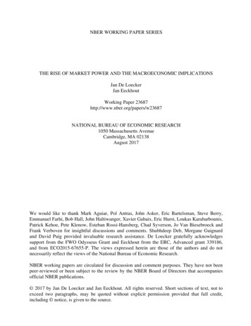
3.1A Secular Trend since 1980Figure 1 presents the weighted average markup, across the economy, over time where weightsare based on firm-level sales. Average markups have gone up since the 1980s. In the beginningof the sample period markups were stable and slightly decreasing from 1.27 in the 1960 to 1.18in 1980. Since 1980 there has been a steady increase to 1.67. In 2014, the average firm charges67% over marginal cost, compared to 18% in 1980. In Appendix B.5 we report some individualfirms’ markups.1.7Markup 10yearFigure 1: The Evolution of Average Markups (1960 - 2014). Average Markup is weighted bymarketshare of sales in the sample.It is well known that the Compustat data is a selected sample and we therefore compareour result to aggregate data from the IRS, and further compare it to the aggregated version ofour data (Compustat). The figures in the Appendix B.4 confirm that these same pattern holds,at the aggregate level, although there is a more modest increase in market power for aggregatedata. The patterns, however, across the (aggregate) Compustat dataset and the economy-wideprivate sector (using IRS) are very similar. This highlights the importance of using micro-leveldata and that industry-level data cannot fully capture the increase in market power. We turnto the micro dimension next.3.2Decomposition: Markups and Firm SizeThe construction of our measure of markup uses weights given by the sales share of the firmin the economy.13 When we compare our measure with the unweighted average of markup13The pattern of aggregate markup depends on the aggregation weight used. The share of Sales is the most common, see for example the HHI index. So far we made no assumption on demand and hence there is no welfaremeasure that guides us which aggregation weight to use. In the Appendix we report aggregate markups for alternative aggregation weights employment and the value of variable inputs. We also report the joint distribution ofthe individual markup and the corresponding weight variable. The pattern of the increase in markups starting in9

in Figure 2a, we observe that the unweighted average is even higher and also increasing morethan our benchmark measure: the unweighted markup goes from 1.4 in 1980 to 2.3 in 2014(and was fairly constant throughout the 1960s and 1970s), compared to an increase from 1.18to 1.67 for the unweighted measure. The fact that the unweighted measure is always higherindicates that larger firms (as measured by their sales) tend to have a lower markup. Thisappears at first to contradict the prediction from models of imperfect competition where firmswith larger market shares have higher markups. Of course, the previous results hold acrossall firms across all sectors, while within narrowly defined industries, however, we confirm thepositive relationship between markups and firm 02010194019601980year20002020yearShare weighted Markupmu meanMarkup(a) Unweighted versus Weighted Markup.Mean 4digit(b) Industry disaggregationFigure 2: Decomposition by market share.We seek to decompose the weighted mean to get at the source of this discrepancy in thelevel with the unweighted measure and to get at what has changed over time that can explainthe rise in markup. If in the total population, large firms have smaller markups, is this alsothe case at more disaggregated levels of industry? Is the change over time due to an overallincrease in markup (the markup tide has been lifting across all industries) or is there a changein the composition of firms of different sizes?We therefore investigate whether this negative relation between markup and sales is due tothe composition of industry or due to the negative relation between size and markup, and usea decomposition method as in Olley and Pakes (1996).T HE CROSS - SECTIONAL DECOMPOSITION . Denote the share sit of firm i’s sales Sit Pit Qit inthe total sales St in the economy (the universe of firms in our sample) by sit SSitt . Then wecan write the weighted markup, denoted by Mt , asXMt sit µiti µt X(sit st )(µit µt )i1980

power is consistent with seven secular trends in the last three decades. While there is ample evidence that market power exists for particular markets and that it is pervasive across sectors, there is surprisingly little systematic evidence of the patterns of mar-ket power across the aggregate economy, and over time. The evidence on market power we