Transcription
An Introduction toLow-Density Parity-Check CodesPaul H. SiegelElectrical and Computer EngineeringUniversity of California, San Diego5/ 31/ 07 egel1
Outline Shannon’s Channel Coding TheoremError-Correcting Codes – State-of-the-ArtLDPC Code Basics EncodingDecodingLDPC Code Design 5/ 31/ 07Asymptotic performance analysisDesign optimizationLDPC Codes2
Outline EXIT Chart AnalysisApplications Binary Erasure ChannelBinary Symmetric ChannelAWGN ChannelRayleigh Fading ChannelPartial-Response ChannelBasic References5/ 31/ 07LDPC Codes3
A Noisy Communication OURCE5/ 31/ 07LDPC Codes4
Channels Binary erasure channel BEC(ε)1- ε0ε0?ε11- ε1 Binary symmetric channel BSC(p)01-ppp0111-p5/ 31/ 07LDPC Codes5
More Channels Additive white Gaussian noise channel AWGNf ( y 1)f ( y 1) P5/ 31/ 07PLDPC Codes6
Shannon CapacityEvery communication channel is characterized bya single number C, called the channel capacity.It is possible to transmit information over thischannel reliably (with probability of error 0)if and only if:# information bitsR Cchannel usedef5/ 31/ 07LDPC Codes7
Channels and CapacitiesC 1 ε Binary erasure channel BEC(ε)1- ε0ε0.80.7?ε1010.90.60.50.40.31- .60.50.4p0.30.211-p5/ 31/ 070.1C 1 H 2 ( p) Binary symmetric channel BSC(p)1-p00.1000.10.20.30.40.50.60.70.80.91H 2 ( p ) p log 2 p (1 p ) log 2 (1 p )LDPC Codes8
More Channels and Capacities Additive white Gaussian noise channel AWGNf ( y 0)f ( y 1)P C log 2 1 2 σ 121.81.6 P1.4P1.210.80.60.40.20-105/ 31/ 07LDPC Codes-8-6-4-202468109
CodingWe use a code to communicate over the noisy channel.Sourcex x1 , x2 , , xkc c1 , c2 , , cnEncoderChannelSinkxˆ xˆ1 , xˆ 2 , , xˆ kCode rate:5/ 31/ 07Decodery y1 , y 2 , , y nR knLDPC Codes10
Shannon’s Coding TheoremsIf C is a code with rate R C, then theprobability of error in decoding this code isbounded away from 0. (In other words, at anyrate R C, reliable communication is notpossible.)For any information rate R C and any δ 0,there exists a code C of length nδ and rate R,such that the probability of error in maximumlikelihood decoding of this code is at most δ.C Max (H(x) – H y (x))5/ 31/ 07Proof: Non-constructive!LDPC Codes11
Review of Shannon’s Paper A pioneering paper:Shannon, C. E. “A mathematical theory of communication. Bell SystemTech. J. 27, (1948). 379–423, 623–656 A regrettable review:Doob, J.L., Mathematical Reviews, MR0026286 (10,133e)“The discussion is suggestive throughout, rather thanmathematical, and it is not always clear that the author’smathematical intentions are honorable.”Cover, T. “Shannon’s Contributions to Shannon Theory,” AMS Notices,vol. 49, no. 1, p. 11, January 2002“Doob has recanted this remark many times, saying that itand his naming of super martingales (processes that go downinstead of up) are his two big regrets.”5/ 31/ 07LDPC Codes12
Finding Good Codes Ingredients of Shannon’s proof: Random code Large block length Optimal decoding ProblemRandomness large block length optimal decoding COMPLEXITY!5/ 31/ 07LDPC Codes13
State-of-the-Art Solution Long, structured, “pseudorandom” codes Practical, near-optimal decoding algorithms Examples Turbo codes (1993) Low-density parity-check (LDPC) codes (1960, 1999) State-of-the-art Turbo codes and LDPC codes have brought Shannon limitsto within reach on a wide range of channels.5/ 31/ 07LDPC Codes14
Evolution of Coding TechnologyLDPCcodes5/ 31/ 07from Trellis and Turbo Coding,Schlegel and Perez, IEEE Press, 2004LDPC Codes15
Linear Block Codes - Basics Parameters of binary linear block code C knRdmin number of information bitsnumber of code bitsk/nminimum distance There are many ways to describe C Codebook (list) Parity-check matrix / generator matrix Graphical representation (“Tanner graph”)5/ 31/ 07LDPC Codes16
Example: (7,4) Hamming Code (n,k)(n,k) (7,4)(7,4),, RR 4/74/7 3 ddminmin 3 singlesingleerrorerrorcorrectingcorrecting doubledoubleerasureerasurecorrectingcorrecting5 EncodingEncodingrule:rule:21.1. 2. of1’s1’sinineacheachcirclecircle5/ 31/ 07LDPC Codes7143617
Example: (7,4) Hamming Code 2k 16 codewords Systematic encoder places input bits in positions 1, 2, 3, 4 Parity bits are in positions 5, 6, 75/ 31/ 070000 0001000 1110001 0111001 1000010 1101010 0010011 1011011 0100100 1011100 0100101 1101101 0010110 0111110 1000111 0001111 111LDPC Codes18
Hamming Code – Parity Checks11 22 33 44 55 66 7751 1 1 0 1 0 0275/ 31/ 071431 0 1 1 0 1 01 1 0 1 0 0 16LDPC Codes19
Hamming Code: Matrix Perspectivec [c1 , c2 , c3 , c4 , c5 , c6 , c7 ] Parity check matrix H 0 TH c 0 0 1 1 1 0 1 0 0 H 1 0 1 1 0 1 0 1 1 0 1 0 0 1 Generator matrix G 1 0G 0 05/ 31/ 070 0 0 1 1 1 1 0 0 1 0 1 0 1 0 1 1 0 0 0 1 0 1 1 u [u1 , u 2 , u3 .u 4 ]c [c1 , c2 , c3 , c4 , c5 , c6 , c7 ]u G cLDPC Codes20
Parity-Check Equations Parity-check matrix implies system of linear equations. 1 1 1 0 1 0 0 H 1 0 1 1 0 1 0 1 1 0 1 0 0 1 c1 c2 c3 c5 0c1 c3 c4 c6 0c1 c2 c4 c7 0 Parity-check matrix is not unique. Any set of vectors that span the rowspace generated by Hcan serve as the rows of a parity check matrix (includingsets with more than 3 vectors).5/ 31/ 07LDPC Codes21
Hamming Code: Tanner Graph Bi-partite graph representing parity-check equationsc1c2c3c4c5c6c75/ 31/ 07c1 c2 c3 c5 0c1 c3 c4 c6 0c1 c2 c4 c7 0LDPC Codes22
Tanner Graph Terminologyvariable nodescheck nodes(bit, left)(constraint, t.5/ 31/ 07LDPC Codes23
Low-Density Parity-Check Codes Proposed by Gallager (1960) “Sparseness” of matrix and graph descriptions Number of 1’s in H grows linearly with block length Number of edges in Tanner graph grows linearly withblock length “Randomness” of construction in: Placement of 1’s in H Connectivity of variable and check nodes Iterative, message-passing decoder Simple “local” decoding at nodes Iterative exchange of information (message-passing)5/ 31/ 07LDPC Codes24
Review of Gallager’s Paper Another pioneering work:Gallager, R. G., Low-Density Parity-Check Codes, M.I.T. Press,Cambridge, Mass: 1963. A more enlightened review:Horstein, M., IEEE Trans. Inform. Thoery, vol. 10, no. 2, p. 172, April1964,“This book is an extremely lucid and circumspect exposition of animportant piece of research. A comparison with other coding anddecoding procedures designed for high-reliability transmission . isdifficult.Furthermore, many hours of computer simulation are neededto evaluate a probabilistic decoding scheme. It appears, however, thatLDPC codes have a sufficient number of desirable features to makethem highly competitive with . other schemes .”5/ 31/ 07LDPC Codes25
Gallager’s LDPC Codes Now called “regular” LDPC codes Parameters (n,j,k) n j k codeword length# of parity-check equations involving each code bitdegree of each variable node# code bits involved in each parity-check equationdegree of each check node Locations of 1’s can be chosen randomly, subject to(j,k) constraints.5/ 31/ 07LDPC Codes26
Gallager’s Construction(n,j,k) (20,3,4) First n/k 5 rows have k 41’s each, descending. Next j-1 2 submatrices ofsize n/k x n 5 x 20 obtainedby applying randomly chosencolumn permutation to firstsubmatrix. Result: jn/k x n 15 x 20parity check matrix for a(n,j,k) (20,3,4) LDPC code.5/ 31/ ----------1 -------------------------------------2 LDPC Codes27
Regular LDPC Code – Tanner Graphn 20 variablenodesnj/k 15 checkright degree k 4left degree j 3nj 60 edgesnj 60 edges5/ 31/ 07LDPC Codes28
Properties of Regular LDPC Codes Design rate: R(j,k) 1 j/k Linear dependencies can increase rate Design rate achieved with high probability as nincreases Example: (n,j,k) (20,3,4) with R 1 3/4 1/4. For j 3, the “typical” minimum distance of codes in the(j,k) ensemble grows linearly in the codeword length n. Their performance under maximum-likelihood decoding onBSC(p) is “at least as good.as the optimum code of asomewhat higher rate.” [Gallager, 1960]5/ 31/ 07LDPC Codes29
Performance of Regular LDPC CodesGallager,Gallager,196319635/ 31/ 07LDPC Codes30
Performance of Regular LDPC CodesGallager,Gallager,196319635/ 31/ 07LDPC Codes31
Performance of Regular LDPC CodesGallager,Gallager,196319635/ 31/ 07LDPC Codes32
Performance of Regular LDPC ,Urbanke,200120016n 10n 106R 1/2R 1/25/ 31/ 07LDPC Codes33
Irregular LDPC Codes Irregular LDPC codes are a natural generalization of Gallager’sLDPC codes. The degrees of variable and check nodes need not be constant. Ensemble defined by “node degree distribution” functions.Λ( x) dv Ρ( x) Λi xidc Ρi x ii 2i 1Ρi number of checkΛ i number of variablenodes of degree inodes of degree i Normalize for fraction of nodes of specified degreeΛ ( x)L( x) Λ (1)5/ 31/ 07P( x)R( x) P(1)LDPC Codes34
Irregular LDPC Codes Often, we use the degree distribution from the edgeperspectiveλ ( x) dv λi x i 1ρ ( x) i 1dc ρ i x i 1i 2λi fraction of edges connectedρ i fraction of edges connectedto check nodes of degree ito variable nodes of degree i Conversion ruleΛ ′(x ) L′(x )λ ( x) Λ ′(1) L′(1)5/ 31/ 07P ′(x ) R ′(x )ρ ( x) P ′(1) R ′(1)LDPC Codes35
Irregular LDPC Codes Design rate i iR (λ , ρ ) 1 λ i iρi 1 i1 ρ ( x ) dx01 λ ( x ) dx0 Under certain conditions related to codewords of weight n/2,the design rate is achieved with high probability as n increases.5/ 31/ 07LDPC Codes36
Examples of Degree Distribution Pairs Hamming (7,4) codeΛ(x ) 3x 3x 2 x 3Ρ(x ) 3 x 4##edgesedges 1212λ (x ) 14 12 x 14 x 2R (λ , ρ ) 1 ρ (x ) x 33 4 7 7 (j,k) – regular LDPC code, length-nΛ(x ) nx jjn kΡ( x ) xk5/ 31/ 07λ (x ) x j 1ρ (x ) x k 1LDPC Codes1/ kjR (λ , ρ ) 1 1 1/ jk37
Encoding LDPC Codes Convert H into equivalent upper triangular form H′1H′ 11011n-k111n-kk(e.g., by Gaussian elimination and column swapping –complexity O(n3) ) This is a “pre-processing” step only.5/ 31/ 07LDPC Codes38
Encoding LDPC Codes Set cn-k 1, ,cn equal to the data bits x1, ,xk . Solve for parities cℓ, ℓ 1, , n-k, in reverse order; i.e.,starting with ℓ n-k, computen kcl Hj l 1kl, jcj Hl , j n kxjj l 1(complexity O(n2) ) Another general encoding technique based upon “approximatelower triangulation” has complexity no more than O(n2), withthe constant coefficient small enough to allow practicalencoding for block lengths on the order of n 105.5/ 31/ 07LDPC Codes39
Linear Encoding Complexity It has been shown that “optimized” ensembles of irregularLDPC codes can be encoded with preprocessing complexity atmost O(n3/2), and subsequent complexity O(n). It has been shown that a necessary condition for the ensemble of(λ, ρ)-irregular LDPC codes to be linear-time encodable isλ ′(0) ρ ′(1) 1 Alternatively, LDPC code ensembles with additional “structure”have linear encoding complexity, such as “irregular repeataccumulate (IRA)” codes.5/ 31/ 07LDPC Codes40
Decoding of LDPC Codes Gallager introduced the idea of iterative, messagepassing decoding of LDPC codes. The idea is to iteratively share the results of localnode decoding by passing them along edges of theTanner graph. We will first demonstrate this decoding method forthe binary erasure channel BEC(ε). The performance and optimization of LDPC codesfor the BEC will tell us a lot about other channels,too.5/ 31/ 07LDPC Codes41
Decoding for the BEC Recall: Binary erasure channel, BEC(ε)1-ε00εxi?ε111-εx (x1, x2, , xn)y (y1, y2, , yn)yitransmitted codewordreceived word Note: if yi {0,1}, then xi yi.5/ 31/ 07LDPC Codes42
Optimal Block Decoding - BEC Maximum a posteriori (MAP) block decoding rule minimizesblock error probability:xˆ MAP ( y ) arg max PX Y ( x y )x C Assume that codewords are transmitted equiprobably.xˆ MAP ( y ) arg max PY X ( y x)x C If the (non-empty) set X(y) of codewords compatible with ycontains only one codeword x, thenxˆ MAP ( y ) x If X(y) contains more than one codeword, then declare a blockerasure.5/ 31/ 07LDPC Codes43
Optimal Bit Decoding - BEC Maximum a posteriori (MAP) bit decoding rule minimizesbit error probability:xˆ iMAP ( y ) arg max PX i Y (b y )b {0 ,1} arg maxb {0 ,1} PX Y( x y)x Cxi b Assume that codewords are transmitted equiprobably. If every codeword x X(y) satisfies xi b, then setxˆ MAP ( y ) b Otherwise, declare a bit erasure in position i.5/ 31/ 07LDPC Codes44
MAP Decoding Complexity Let E {1, ,n} denote the positions of erasures in y, and letF denote its complement in {1, ,n}. Let wE and wF denote the corresponding sub-words of word w. Let HE and HF denote the corresponding submatrices of theparity check matrix H. Then X(y), the set of codewords compatible with y, satisfiesX( y ) { x C xF yF and H E xET H F yFT} So, optimal (MAP) decoding can be done by solving a set oflinear equations, requiring complexity at most O(n3). For large blocklength n, this can be prohibitive!5/ 31/ 07LDPC Codes45
Simpler Decoding We now describe an alternative decoding procedurethat can be implemented very simply. It is a “local” decoding technique that tries to fill inerasures “one parity-check equation at a time.” We will illustrate it using a very simple and familiarlinear code, the (7,4) Hamming code. We’ll compare its performance to that of optimal bitwise decoding. Then, we’ll reformulate it as a “message-passing”decoding algorithm and apply it to LDPC codes.5/ 31/ 07LDPC Codes46
Local Decoding of Erasures dmin 3, so any two erasures can beuniquely filled to get a codeword. Decoding can be done locally:Given any pattern of one or twoerasures, there will always be aparity-check (circle) involvingexactly one erasure. The parity-check represented by thecircle can be used to fill in the erasedbit.5271436 This leaves at most one more erasure.Any parity-check (circle) involving itcan be used to fill it in.5/ 31/ 07LDPC Codes47
Local Decoding - Example All-0’s codeword transmitted. Two erasures as shown.0 Start with either the red parityor green parity circle. The red parity circle requiresthat the erased symbol inside itbe 0.5/ 31/ 07LDPC Codes?00?0048
Local Decoding -Example Next, the green parity circle orthe blue parity circle can beselected.0 Either one requires that theremaining erased symbol be 0.005/ 31/ 07LDPC Codes0?0049
Local Decoding -Example Estimated codeword:[0 0 0 0 0 0 0] Decoding successful!! This procedure would haveworked no matter whichcodeword was transmitted.5/ 31/ 070LDPC Codes00000050
Decoding with the Tanner Graph:an a-Peeling Decoder Initialization: Forward known variable nodevalues along outgoing edges Accumulate forwarded values atcheck nodes and “record” theparity Delete known variable nodes andall outgoing edges5/ 31/ 07LDPC Codes51
Peeling Decoder – Initialization5/ 31/ 07xx00?00?00?11LDPC CodesForwardForwardknownknownvaluesvalues52
Peeling Decoder - InitializationxxAccumulate parity00?00?00?115/ 31/ 07LDPC CodesDelete known variablenodes and edges53
Decoding with the Tanner Graph:an a-Peeling Decoder Decoding step: Select, if possible, a check node with one edge remaining;forward its parity, thereby determining the connectedvariable node Delete the check node and its outgoing edge Follow procedure in the initialization process at the knownvariable node Termination If remaining graph is empty, the codeword is determined If decoding step gets stuck, declare decoding failure5/ 31/ 07LDPC Codes54
Peeling Decoder – Step 1x0Find degree-1 check node;forward accumulated parity;determine variable node valuex00000?00?115/ 31/ 07LDPC CodesDelete check node and edge;forward new variable node value55
Peeling Decoder – Step 1xAccumulate parityx000000?00?115/ 31/ 07LDPC CodesDelete known variablenodes and edges56
Peeling Decoder – Step 2xFind degree-1 check node;forward accumulated parity;determine variable node valuex0000001100?115/ 31/ 07LDPC CodesDelete check node and edge;forward new variable node value57
Peeling Decoder – Step 2xAccumulate parityx0000001100?115/ 31/ 07LDPC CodesDelete known variablenodes and edges58
Peeling Decoder – Step 3xFind degree-1 check node;forward accumulated parity;determine variable node valuex000000110011115/ 31/ 07LDPC CodesDelete check node and edge;decoding complete59
Message-Passing Decoding The local decoding procedure can bedescribed in terms of an iterative,“message-passing” algorithm inwhich all variable nodes and allcheck nodes in parallel iterativelypass messages along their adjacentedges. The values of the code bits areupdated accordingly. The algorithm continues until allerasures are filled in, or until thecompletion of a specified number ofiterations.5/ 31/ 07LDPC Codes60
Variable-to-Check Node Messageu?from channelv uuu ?v ?edgeedge eeedgeedge ee?Variable-to-check message on edge eIf all other incoming messages are ?, send message v ?If any other incoming message u is 0 or 1, send v u and,if the bit was an erasure, fill it with u, too.(Note that there are no errors on the BEC, so a message thatis 0 or 1 must be correct. Messages cannot be inconsistent.)5/ 31/ 07LDPC Codes61
Check-to-Variable Node Messageu ?u v1 v2 v3v1edgeedge eeedgeedge eev1v2v2v3Check-to-variable message on edge eIf any other incoming message is ?, send u ?If all other incoming messages are in {0,1},send the XOR of them, u v1 v2 v3.5/ 31/ 07LDPC Codes62
Message-Passing Example – Initializationyyxx yy0000 00? ?0000 00? ?0000 00? ?1111 115/ 31/ 07LDPC CodesVariable-to-CheckVariable-to-Check63
Message-Passing Example – Round 1x yx yCheck-to-Variable0 00 0? ?0 ?0 00 0? ? ?0 00 0? ? ?1 11 15/ 31/ 07LDPC CodesVariable-to-Check64
Message-Passing Example – Round 2x yx yCheck-to-Variable0 00 00 ?0 ?0 00 0? ?1 ?0 00 0? ? ?1 11 15/ 31/ 07LDPC CodesVariable-to-Check65
Message-Passing Example – Round 3x yx yCheck-to-Variable0 00 00 ?0 ?0 00 01 ?1 ?0 00 0? ?1 ?1 11 15/ 31/ 07LDPC CodesVariable-to-CheckDecoding complete66
Sub-optimality of Message-Passing DecoderHamming code: decoding of 3 erasures There are 7 patterns of 3 erasures thatcorrespond to the support of a weight-3codeword. These can not be decoded byany decoder!0 The other 28 patterns of 3 erasures can beuniquely filled in by the optimal decoder. We just saw a pattern of 3 erasures thatwas corrected by the local decoder. Arethere any that it cannot? Test:5/ 31/ 07?0?0?1?0 010LDPC Codes67
Sub-optimality of Message-Passing Decoder Test:?0 0100 There is a unique way to fill theerasures and get a codeword:1100 010The optimal decoder would find it.101001 But every parity-check has at least 2erasures, so local decoding will notwork!5/ 31/ 07LDPC Codes68
Stopping Sets A stopping set is a subset S of the variable nodes suchthat every check node connected to S is connected toS at least twice. The empty set is a stopping set (trivially). The support set (i.e., the positions of 1’s) of anycodeword is a stopping set (parity condition). A stopping set need not be the support of a codeword.5/ 31/ 07LDPC Codes69
Stopping Sets Example 1: (7,4) Hamming codeCodewordsupport setS {4,6,7}5/ 31/ 0712345670001011LDPC Codes70
Stopping Sets Example 2: (7,4) Hamming code15/ 31/ 072345LDPC Codes6771
Stopping Sets Example 2: (7,4) Hamming codeNot the supportset of a codewordS {1,2,3}15/ 31/ 072345LDPC Codes6772
Stopping Set Properties Every set of variable nodes contains a largest stopping set(since the union of stopping sets is also a stopping set). The message-passing decoder needs a check node withat most one edge connected to an erasure to proceed. So, if the remaining erasures form a stopping set, the decodermust stop. Let E be the initial set of erasures. When the messagepassing decoder stops, the remaining set of erasures is thelargest stopping set S in E. If S is empty, the codeword has been recovered. If not, the decoder has failed.5/ 31/ 07LDPC Codes73
Suboptimality of Message-Passing Decoder An optimal (MAP) decoder for a code C on the BECfails if and only if the set of erased variables includesthe support set of a codeword. The message-passing decoder fails if and only the setof erased variables includes a non-empty stopping set. Conclusion: Message-passing may fail where optimaldecoding succeeds!!Message-passing is suboptimal!!5/ 31/ 07LDPC Codes74
Comments on Message-Passing Decoding Bad news: Message-passing decoding on a Tanner graph isnot always optimal. Good news: For any code C, there is a parity-check matrix onwhose Tanner graph message-passing is optimal,e.g., the matrix of codewords of the dual code C . Bad news: That Tanner graph may be very dense, so evenmessage-passing decoding is too complex.5/ 31/ 07LDPC Codes75
Another (7,4) Code 1 1 0 1 0 0 0 H 0 0 1 1 0 1 0 0 0 0 1 1 0 1 R 4/7dmin 2All stopping sets contain codeword supports.Message-passing decoder on this graph is optimal!(Cycle-free Tanner graph implies this.)5/ 31/ 07LDPC Codes76
Comments on Message-Passing Decoding Good news: If a Tanner graph is cycle-free, the messagepassing decoder is optimal! Bad news: Binary linear codes with cycle-free Tanner graphsare necessarily weak. Good news: The Tanner graph of a long LDPC code behavesalmost like a cycle-free graph!5/ 31/ 07LDPC Codes77
Analysis of LDPC Codes on BEC In the spirit of Shannon, we can analyze theperformance of message-passing decoding onensembles of LDPC codes with specified degreedistributions (λ,ρ). The results of the analysis allow us to design LDPCcodes that transmit reliably with MP decoding at ratesapproaching the Shannon capacity of the BEC. In fact, sequences of LDPC codes have been designedthat actually achieve the Shannon capacity. The analysis can assume the all-0’s codeword is sent.5/ 31/ 07LDPC Codes78
Key Results - 1 Concentration With high probability, the performance of ℓ roundsof MP decoding on a randomly selected (n, λ, ρ)code converges to the ensemble averageperformance as the length n . Convergence to cycle-free performance The average performance of ℓ rounds of MPdecoding on the (n, λ, ρ) ensemble converges to theperformance on a graph with no cycles of length 2ℓ as the length n .5/ 31/ 07LDPC Codes79
Key Results - 2 Computing the cycle-free performance The cycle-free performance can be computed by atractable algorithm – density evolution. Threshold calculation There is a threshold probability p*(λ,ρ) such that,for channel erasure probability ε p*(λ,ρ), thecycle-free error probability approaches 0 as thenumber of iterations ℓ .5/ 31/ 07LDPC Codes80
Asymptotic Performance Analysis We assume a cycle-free (λ,ρ) Tanner graph. Let p0 ε, the channel erasure probability. We find a recursion formula for pℓ , theprobability that a randomly chosen edge carries avariable-to-check erasure message in round ℓ. We then find the largest ε such that pℓ convergesto 0, as ℓ . This value is called the threshold. This procedure is called “density evolution”analysis.5/ 31/ 07LDPC Codes81
Density Evolution-1 messages.messages.Pr (u ? ) Pr (vi ?, for some i 1, , d 1) 1 Pr (vi ?, for all i 1, , d 1) 1 (1 p 1 )1d 1 The probability that edge e connects toa check node of degree d is ρd , soPr (u ?) dc uu edge ev edge eρ d (1 (1 p 1 ) d 1 )vd 2vd 1d 1 1 dc ρ d (1 p 1 ) d 1d 1 1 ρ (1 p5/ 31/ 07 1)LDPC Codes82
Density Evolution-2vvedgeedge eeu0from channelu1ud 2u d 1 Consider a variable node of degreed with independent incomingmessages.Pr (v ?) Pr (u 0 ?) Pr (ui ?, for all i 1, , d 1) p0 [1 ρ (1 p 1 ) ]d 1 The probability that edge e connects toa variable node of degree d is λd , soPr (v ?) dv λd p0 [1 ρ (1 pd 1 p0 λ (1 ρ (1 p 1d 1)] 1))pℓ p0 λ (1–ρ(1–pℓ-1))5/ 31/ 07LDPC Codes83
Threshold Propertypℓ p0 λ (1–ρ(1–pℓ-1)) There is a threshold probability p*(λ, ρ) such thatifthenp0 ε p * (λ , ρ ),lim p 0. 5/ 31/ 07LDPC Codes84
Threshold Interpretation Operationally, this means that using a code drawnfrom the ensemble of length-n LDPC codes withdegree distribution pair (λ, ρ), we can transmit asreliably as desired over the BEC(ε) channel ifε p * (λ , ρ ) ,for sufficiently large block length n .5/ 31/ 07LDPC Codes85
Computing the Threshold Define f (p,x) p λ (1–ρ(1–x)) The threshold p*(λ, ρ) is the largest probability p suchthatf (p,x) – x 0on the interval x (0,1]. This leads to a graphical interpretation of thethreshold p*(λ, ρ)5/ 31/ 07LDPC Codes86
Graphical Determination of the Threshold Example: (j,k) (3,4)(f ( x, p ) x p 1 (1 x))3 2 xp* 0.6474p 0.7p 0.6474p 0.6p 0.55/ 31/ 07LDPC Codes87
(j,k)-Regular LDPC Code Thresholds There is a closed form expression for thresholds of(j,k)-regular LDPC codes. Examples:5/ 31/ 07(j,k)(3,4)(3,5)(3,6)(4,6)R1/42/51/21/3pSh¾ 0.753/5 0.6½ 0.5⅔ 0.67p*(j,k) 0.6474 0.5176 0.4294 0.5061(4,8)1/2½ 0.5 0.3834LDPC Codesp * (3,4) 31253672 252 21 0.64742688
Degree Distribution Optimization Two approaches: Fix design rate R(λ,ρ) and find degreedistributions λ(x), ρ(x) to maximize the thresholdp*(λ,ρ). Fix the threshold p*, and find degree distributionsλ(x), ρ(x) to maximize the rate R(λ,ρ). For the latter, we can: start with a specific ρ(x) and optimize λ(x); then, for the optimal λ(x), find the optimal checkdistribution; ping-pong back and forth until satisfied with theresults.5/ 31/ 07LDPC Codes89
Variable Degree Distribution Optimization Fix a check degree distribution ρ(x) and threshold ε. Fix maximum variable degree lmax . Defineg ( x, λ2 , , λl max ) ελ (1 ρ (1 x)) x ε λ (1 ρ (1 x))ii 1 xi 2 Use linear programming to findl max lmax max (λi / i ) λi 0; λi 1; g 0 for x [0,1] λ i 2 i 2 Since the rate R(λ,ρ) is an increasing function of λi/i,this maximizes the design rate.5/ 31/ 07LDPC Codes90
Practical Optimization In practice, good performance is found for a check degreedistribution of the form:ρ ( x) ax r 1 (1 a) x r Example 1: lmax 8, r 6, design rate ½λ ( x) 0.409 x 0.202 x 2 0.0768 x 3 0.1971x 6 0.1151x 7ρ ( x) x 5 Rate: Threshold:5/ 31/ 07R(λ,ρ) 0.5004p*(λ,ρ) 0.4810LDPC Codes91
Bound on the Threshold Taylor series analysis yields the general upper bound:1p * (λ , ρ ) .λ ′(0) ρ ′(1) For previous example with p*(λ,ρ) 0.4810, the upper boundgives:11 0.4890λ ′(0) ρ ′(1) (0.409) 55/ 31/ 07LDPC Codes92
EXIT Chart Analysis Extrinsic information transfer (EXIT) charts provide a nicegraphical depiction of density evolution and MP decoding[tenBrink,1999] Rewrite the density evolution recursion as:f ( x, p ) pλ (1 ρ (1 x)) v p (c( x))wherev p ( x ) pλ ( x )c( x) 1 ρ (1 x)5/ 31/ 07LDPC Codes93
EXIT Chart Analysis Recall that the MP convergence condition wasf ( x, p ) x, for all x (0,1) Since λ(x) is invertible, the condition becomes 1c( x) v p ( x), for all x (0,1) Graphically, this says that the curve for c(x) must lie 1below the curve for v p ( x) for all p p*.5/ 31/ 07LDPC Codes94
EXIT Chart Example Example: (3,4)-regular LDPC code, p* 0.6474λ ( x) x 2v p ( x) pλ ( x)ρ ( x) x 3c( x) 1 ρ (1 x) px 2 x v ( x) p 1p5/ 31/ 07 1 (1 x) 312LDPC Codes95
EXIT Chart Example Example: (3,4)-regular LDPC code, p* 0.647410.9p 0.5p 0.60.8 x v p1 ( x) p p 0.7p 0.80.70.6for variousvalues ofinitial erasureprobability p0.5p* 0.64740.4120.3c( x) 1 (1 x) 30.20.105/ 31/ 0700.10.20.30.40.50.6LDPC Codes0.70.80.9196
EXIT Charts and Density Evolution EXIT charts can be used to visualize densityevolution. Assume initial fraction of erasure messages p0 p. The fraction of erasures emitted successively by checknode qi and by variable nodes and pi are obtained bysuccessively applying c(x) and vp(x).q1 c( p0 )p1 v p (q1 ) v p (c( p0 ))[note : v p1 ( p1 ) q1 ]q 2 c( p1 )p 2 v p (q 2 ) v p (c( p1 ))5/ 31/ 07LDPC Codes[note : v p1 ( p 2 ) q 2 ]97
EXIT Charts and Density Evolution Graphically, this computation describes a staircasefunction. If p p*, there is a “tunnel” between vp-1(x) and c(x)through which the staircase descends to ground level,i.e., no erasures. If p p*, the tunnel closes, stopping the staircasedescent at a positive fraction of errors.5/ 31/ 07LDPC Codes98
Density Evolution Visualization - 1 Example: (3,4)-regular LDPC code, p 0.61 x v0 .16 ( x) 0.6 0.90.8120.70.6c( x) 1 (1 x) 30.50.40.30.20.105/ 31/ 0700.10.20.30.40.50.6LDPC Codes0.70.80.9199
Density Evolution Visualization-2 Example: (3,4)-regular LDPC code1p0 0.60.9qfrac
Review of Shannon's Paper 5/ 31/ 07 LDPC Codes 12 A pioneering paper: Shannon, C. E. "A mathematical theory of communication. Bell System Tech. J. 27, (1948). 379-423, 623-656 A regrettable review: