WIXLIB

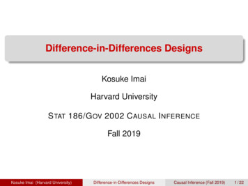
Difference-in-Differences DesignsKosuke ImaiHarvard UniversityS TAT 186/G OV 2002 C AUSAL I NFERENCEFall 2019Kosuke Imai (Harvard University)Difference-in-Differences DesignsCausal Inference (Fall 2019)1 / 22

MotivationHow should we conduct causal inference when repeatedmeasurements are available?Two types of variations:12cross-sectional variation within each time periodtemporal variation within each unit1.01.0Before-and-after and cross-sectional designs0.80.6 counterfactual counterfactualcontrol group0.2 0.2treatment group0.4 Average Outcome0.6 0.4Average Outcome0.8treatment groupcontrol group0.0 0.0 time ttime t 1time ttime t 1Can we exploit both variations?Kosuke Imai (Harvard University)Difference-in-Differences DesignsCausal Inference (Fall 2019)2 / 22

Minimum Wage and Unemployment(Card and Krueger. 1994. Am. Econ. Rev)How does the increase in minimum wage affect employment?Many economists believe the effect is negativeespecially for the pooralso for the whole economyHard to randomize the minimum wage increaseIn 1992, NJ minimum wage increased from 4.25 to 5.05Neighboring PA stays at 4.25Observe employment in both states before and after increaseNJ and (eastern) PA are similarFast food chains in NJ and PA are similar: price, wages, products,etc.They are most likely to be affected by this increaseKosuke Imai (Harvard University)Difference-in-Differences DesignsCausal Inference (Fall 2019)3 / 22

nce-in-Differences0.340.32treatment group(New Jersey)control group(Pennsylvania) averagecausal effectestimate 0.280.30 0.26 counterfactual(New Jersey)0.24Average Proportion of Full time Employees0.36Parallel trend assumptionbeforeKosuke Imai (Harvard University)afterDifference-in-Differences DesignsCausal Inference (Fall 2019)4 / 22

Setup:Two time periods: time 0 (pre-treatment), time 1 (post-treatment)Gi : treatment (Gi 1) or control (Gi 0) groupZit tGi : treatment assignment indicator for t 0, 1Potential outcomes: Yi0 (0), Yi0 (1), Yi1 (0), Yi1 (1)Observed outcomes: Yit Yit (Zit )Average treatment effect for the treated:τ E{Yi1 (1) Yi1 (0) Gi 1}Parallel trend assumption:E{Yi1 (0) Yi0 (0) Gi 1} E{Yi1 (0) Yi0 (0) Gi 0}DiD estimator:τ̂DiD {E(Yi1 Gi 1) E(Yi0 Gi 1)} {E(Yi1 Gi 0) E(Yi0 Gi 0)}Applicable to repeated cross-section data as wellKosuke Imai (Harvard University)Difference-in-Differences DesignsCausal Inference (Fall 2019)5 / 22

Linear Model for the Difference-in-DifferencesTwo-way fixed effects model:Yit (z) αi βt τ z itE{Yi0 (0)} αiE{Yi1 (0)} αi βE{Yi1 (1)} αi β τE{Yi1 (1) Yi1 (0)} τParallel trend assumption:E{Yi1 (0) Yi0 (0) Gi g} βOr equivalently E( i1 i0 Gi g) 0Both Zit and it can depend on αi or unobserved confoundersLeast squares estimator equals the nonparametric DiD estimator,i.e., τ̂FE τ̂DiDThis equivalence does not hold in general beyond the 2 2 caseKosuke Imai (Harvard University)Difference-in-Differences DesignsCausal Inference (Fall 2019)6 / 22

Comparison with the Lagged Outcome ModelLagged outcome model:Yi1 (z) α ρYi0 τ z i (z)Nonparametric identification assumption:{Yi1 (1), Yi1 (0)} Zit Yi0can be made conditional on Xi as well as Yi0neither stronger nor weaker than the parallel trend assumptionsame as parallel trend if E(Yi0 Gi 1) E(Yi0 Gi 0)Where does the imbalance in lagged outcome come from?Difference-in-Differencesunobserved time-invariant confounderLagged outcome directly affects treatment assignmentKosuke Imai (Harvard University)Difference-in-Differences DesignsCausal Inference (Fall 2019)7 / 22

Relationship between the DiD and Lagged OutcomeEstimatorsLeast squares estimator:τ̂LD E(Yi1\ Gi 1) E(Yi1\ Gi 0) ρ̂{(E(Yi0\ Gi 1) E(Yi0\ Gi 0))}If ρ̂ 1, then τ̂LD τ̂DiDAssume 0 ρ 1 (stationarity)Without loss of generality, assume E(Yi0 Gi 1) E(Yi0 Gi 0)(monotonicity)12If parallel trend holds, E(τ̂LD ) E(τ̂DiD ) τIf ignorability holds, τ E(τ̂LD ) E(τ̂DiD )Nonparametric estimator (Ding and Li. 2019. Political Anal.):µ0 E{Yi1 (0) Gi 1} E{E(Yi1 Gi 0, Yi0 ) Gi 1}(stationarity) E(Yi1 Gi 0, Yi0 y )/ y 1 for all y(stochastic monotonicity) FY0 (y Gi 1) FY0 (y Gi 0) for all yThen, the bracketing relationship holdsKosuke Imai (Harvard University)Difference-in-Differences DesignsCausal Inference (Fall 2019)8 / 22

Adjusting for Baseline CovariatesParallel trend assumption conditional on the baseline covaraites:E{Yi1 (0) Yi0 (0) Xi x, Gi 1} E{Yi1 (0) Yi0 (0) Xi x, Gi 0} for all xMatching: parallel trend within a pair or a strataWeighting (Abadie. 2005. Rev. Econ. Stud ):E{Yi1 (1) Yi1 (0) Gi 1} Yi1 Yi0 Gi Pr(Gi 1 Xi ) E·Pr(Gi 1) 1 Pr(Gi 1 Xi )Unconditional parallel trend assumption neither implies nor isimplied by conditional parallel trend assumptionKosuke Imai (Harvard University)Difference-in-Differences DesignsCausal Inference (Fall 2019)9 / 22

Nonlinear Difference-in-Differences(Athey and Imbens. 2006. Econometrica )Standard DiD relies upon the linearity assumptionNot invariant to a nonlinear transformation of outcome (e.g., log)ControlTreated11qqF00r0 (q)r1 (q)F01F100F110 4 2024 4 2024Temporal change in quantile is identical between the two groupsKosuke Imai (Harvard University)Difference-in-Differences DesignsCausal Inference (Fall 2019)10 / 22

Formalization of Nonlinear DiDDistribution functions: Fgt (y ) Pr(Yit (0) y Gi g)Quantile treatment effect for a given q:e 1 (q) F 1 (q)τ (q) F1111e11 (y ) Pr(Yi1 (1) y Gi 1)where FWe wish to identify F11 (y )Identification assumption: 1 1F01 (F00(q)) F11 (F10(q)) {z} {z}r0 (q)r1 (q)for all q [0, 1]Under this assumption, 1F11 (y ) F01 [F00{F10 (y )}]Kosuke Imai (Harvard University)Difference-in-Differences DesignsCausal Inference (Fall 2019)11 / 22

Synthetic Control Method (Abadie et al. 2010. J. Am. Stat. Assoc.)One treated unit i 1 receiving the treatment at time TQuantity of interest: Y1T Y1T (0)Create a synthetic control using past outcomesWeighted average:Y\1T (0) NXŵi YiTi 2where the weights balance past outcomesŵ argminT 1XwwithPNi 2 ŵit 1Y1t NX!2wi Yiti 2 1 and ŵi 0One could include time-invariant covariates XiKosuke Imai (Harvard University)Difference-in-Differences DesignsCausal Inference (Fall 2019)12 / 22

Causal Effect of ETA’s TerrorismTHE AMERICAN ECONOMIC REVIEW-5MARCH 200311-/s/a210-/509-,-Actual with terrorism- -Synthetic without terrorism11955 1960 1965 1970 1975 1980 1985 1990 1995 2000yearFIGURE1. PERCAPITA GDPFOR THEBASQUECOUNTRI(Abadie and Gardeazabal. 2003. Am. Econ. Rev.)4\Kosuke Imai (Harvard University)- - GDt' gapCausal Inference (Fall 2019)Difference-in-Differences Designs13 / 22

Placebo TestTHE AMERICAN ECONOMIC REVIEWMARCH 2003Actual without terrorismSynthetic without terrorism3)75 1980 1985 1990 1995 2000yearFIGURE4 A "PLACEBOSTUDY."PERCAPITAGDPFORCATALONIAthe allmaincontrolcontributorto theandsyn- compareeconomic effectof withterrorismthe Basqueunitcan Cataloniado thisisforunitsthemtheon treatedCountry. To the extent that the regions whichthetic control for the Basque Country, an 9)form Designsthe synthetic controlhave(Fallbeenecoper capitaGDP forKosukeImai (Harvardnormallyhigh University)level of14 / 22

Kosuke Imai (Harvard University)Difference-in-Differences DesignsCausal Inference (Fall 2019)15 / 22

Model-based JustificationThe main motivating factor analytic model:Yit (0) γt δt Xi ξt Ui itGeneralization of the linear two-way fixed effects modelKey assumption: there exist weights such thatNXi 2wi Xi X1andNXwi Ui U1i 2Another motivating autoregressive model with time-varyingcovariates:Yit (0) ρt Yi,t 1 (0) δt Xit itXit λt 1 Yi,t 1 (0) t 1 Xi,t 1 νitPast outcomes can affect current treatmentNo unobserved time-invariant confoundersKosuke Imai (Harvard University)Difference-in-Differences DesignsCausal Inference (Fall 2019)16 / 22

Generalizing the Difference-in-Differencesstaggered treatmentWhat if units go in and out of treatment?Democracy as the TreatmentWar as the Treatmentgermanyaustraliakoreacanadaitalynew tAutocracy (Control)190019502000YearDemocracy (Treatment)Acemoglu et al. 2019. J. Political Econ.treatmentPeace (Control)War (Treatment)Scheve and Stasavage. 2012.Am. Political Sci. Rev.Kosuke Imai (Harvard University)Difference-in-Differences DesignsCausal Inference (Fall 2019)17 / 22

Matching Methods for Panel Data (Imai et al. 2019. Working Paper)Choose the number of lags L and leads FATE of Policy Change for the Treated:n E Yi,t F Zit 1, Zi,t 1 0, {Zi,t }L 2 oYi,t F Zit 0, Zi,t 1 0, {Zi,t }L 2 Zit 1, Zi,t 1 0Estimation procedure:Construct a matched set for each treated unit that consists ofcontrol units with the identical treatment history up to L time periods2Refine covariate balance with a matching/weighting method withina matched set3Use the multi-period difference-in-differences estimator: N TX F XX01Zit (Yi,t F Yi,t 1 ) witi (Yi 0 ,t F Yi 0 ,t 1 )PT F Zit01PNi 1t L 1i Miti 1 t L 1Kosuke Imai (Harvard University)Difference-in-Differences DesignsCausal Inference (Fall 2019)18 / 22

Empirical Application (1)ATT with L 4 and F 1, 2, 3, 4We consider democratization and authoritarian reversalExamine the number of matched control units18 (13) treated observations have no matched control30Authoritarian Reversal25Four Year Lags 5 Emtpy SetsOne Year Lag 0 Emtpy Sets05Frequency10 15 2025Frequency10 15 2050Acemoglu et al. (2018)30DemocratizationFour Year Lags 9 Emtpy SetsOne Year Lag 0 Emtpy Sets0204060801001200Kosuke Imai (Harvard University)3025Four Year Lags 2 Emtpy SetsOne Year Lag 0 Emtpy Sets20406080100120Ending Warncy203025ncy20vage (2012)Starting WarDifference-in-Differences DesignsFour Year Lags 18 Emtpy SetsOne Year Lag 17 Emtpy SetsCausal Inference (Fall 2019)19 / 22

Improved Covariate Balance 120 1 2 3 2 1 4 3 2 1 4 3 2 1 4 3 2 1 4 3 2 1 3 2CausalInference(Fall 42019) 1 1 4 3 2 1Difference-in-DifferencesDesigns1012 2 101 1 2012 2 1012 201 1 221120 1 2 3 4 1 2 4Propensity ScoreWeighting 2 3 12 4 22 1 31 20 1 2 4 3 2 1Kosuke Imai(HarvardUniversity)120 1 2 3010 1 221 10 4 40 1 1 1 2 2 2 3 32 4 4 1 1Propensity ScoreMatching 2 22 32 4Mahalanobis DistanceMatching1210 1 2 2 1012BeforeRefinement 2Standardized MeanDifferences forDemocratizationStandardized MeanDifferences forAuthoritarian ReversalStandardized MeanDifferences forStarting Warcheve & Stasavage (2012)Acemoglu et al. (2018)BeforeMatching20 / 22

Estimated Causal EffectsMahalanobis MatchingUp to 10 matchesPropensity ScoreWeighting0.050.15Up to 5 matches 4 40 123 123401234 231234 0.1 123 0123 400.050.150 0.1 0.2Estimated Effect ofAuthoritarian ReversalPropensity Score MatchingUp to 10 matches 0.2Estimated Effect ofDemocratizationUp to 5 matches0123401234012340140Years relative to the administration of treatmentKosuke Imai (Harvard University)Difference-in-Differences DesignsCausal Inference (Fall 2019)21 / 22

Concluding RemarksDifference-in-differences design:fully exploit the panel data structurecross sectional and before-and-after designs do notparallel trend assumptionadjusts for time-invariant unobserved confounderstradeoff between dynamics and unobservablesExtensions:adjusting for baseline covariatesnonlinear difference-in-differencessysthetic controlsmultiperiod difference-in-differences estimatorReadings: A NGRIST AND P ISKE . C HAPTER 5Kosuke Imai (Harvard University)Difference-in-Differences DesignsCausal Inference (Fall 2019)22 / 22

Figure 4. Per-capita cigarette sales gaps in California and placebo gaps in all 38 control states. provide a good Þt for per capita cigarette consumption prior to Proposition 99 for the majority of the states in the donor pool. However, Figure 4 indicates also that per capita cigarette sales during the 1970Ð1988 period cannot be well reproduced