WIXLIB

Mixtures of Probabilistic Principal Component Analysers2.24Factor AnalysisPerhaps the most common example of a latent variable model is that of statistical factor analysis(Bartholomew 1987), in which the mapping y(x; w) is a linear function of x:t Wx µ ².(2)Conventionally, the latent variables are defined to be independent and Gaussian with unit variance,so x N (0, I). The noise model is also Gaussian such that ² N (0, Ψ), with Ψ diagonal, andthe (d q) parameter matrix W contains the factor loadings. The parameter µ permits the datamodel to have non-zero mean. Given this formulation, the observation vectors are also normallydistributed t N (µ, C), where the model covariance is C Ψ WWT . (Note that as a resultof this parameterisation C is invariant under post-multiplication of W by an orthogonal matrix,equivalent to a rotation of the x co-ordinate system.) The key motivation for this model is that,because of the diagonality of Ψ, the observed variables t are conditionally independent given thelatent variables, or factors, x. The intention is that the dependencies between the data variablest are explained by a smaller number of latent variables x, while ² represents variance unique toeach observation variable. This is in contrast to conventional PCA, which effectively treats bothvariance and covariance identically. It should also be noted that there is no closed-form analyticsolution for W and Ψ, and so their values must be determined by iterative procedures.2.3Links from Factor Analysis to PCAIn factor analysis the subspace defined by the columns of W will generally not correspond to theprincipal subspace of the data. Nevertheless, certain links between the two methods have previouslybeen noted. For instance, it has been observed that the factor loadings and the principal axes arequite similar in situations where the estimates of the elements of Ψ turn out to be approximatelyequal (e.g. Rao 1955). Indeed, this is an implied result of the fact that if Ψ σ 2 I and an isotropic,rather than diagonal, noise model is assumed, then PCA emerges if the d q smallest eigenvaluesof the sample covariance matrix S are exactly equal. This “homoscedastic residuals model” isconsidered by Basilevsky (1994, p361), for the case where the model covariance is identical toits data sample counterpart. Given this restriction, the factor loadings W and noise variance σ 2are identifiable (assuming correct choice of q) and can be determined analytically through eigendecomposition of S, without resort to iteration (Anderson 1963).However, this established link with PCA requires that the d q minor eigenvalues of the samplecovariance matrix be equal (or more trivially, be negligible) and thus implies that the covariancemodel must be exact. Not only is this assumption rarely justified in practice, but when exploitingPCA for dimensionality reduction, we do not require an exact characterisation of the covariancestructure in the minor subspace, as this information is effectively ‘discarded’. In truth, what is ofreal interest in the homoscedastic residuals model is the form of the maximum-likelihood solutionwhen the model covariance is not identical to its data sample counterpart.Importantly, we show in the following section that PCA does still emerge in the case of an approximate model. In fact, this link between factor analysis and PCA had been partially explored in theearly factor analysis literature by Lawley (1953) and Anderson and Rubin (1956). Those authorsshowed that the maximum-likelihood solution in the approximate case was related to the eigenvectors of the sample covariance matrix, but did not show that these were the principal eigenvectorsbut instead made this additional assumption. In the next section (and Appendix A) we extend thisearlier work to give a full characterisationof the properties of the model we term “probabilistic¡ PCA”. Specifically, with ² N 0, σ 2 I , the columns of the maximum-likelihood estimator WMLare shown to span the principal subspace of the data even when C 6 S.

Mixtures of Probabilistic Principal Component Analysers35Probabilistic PCA3.1The Probability Model¡ For the case of isotropic noise ² N 0, σ 2 I , equation (2) implies a probability distribution overt-space for a given x of the form½¾1p(t x) (2πσ 2 ) d/2 exp 2 kt Wx µk2 .(3)2σWith a Gaussian prior over the latent variables defined by½¾1 T q/2p(x) (2π)exp x x ,2we obtain the marginal distribution of t in the formZp(t) p(t x)p(x)dx,½¾1 1/2 d/2T 1 (2π) C exp (t µ) C (t µ) ,2where the model covariance isC σ 2 I WWT .(4)(5)(6)(7)Using Bayes’ rule, the posterior distribution of the latent variables x given the observed t may becalculated:p(x t) (2π) q/2 σ 2 M 1/2 · ªT ª1 exp x M 1 WT (t µ) (σ 2 M) x M 1 WT (t µ) ,2(8)where the posterior covariance matrix is given byσ 2 M 1 σ 2 (σ 2 I WT W) 1 .(9)Note that M is q q while C is d d.The log-likelihood of observing the data under this model isL NXln {p(tn )} ,n 1 ¡ ªN d ln(2π) ln C tr C 1 S ,2whereS N1 X(tn µ)(tn µ)T ,N n 1(10)(11)is the sample covariance matrix of the observed {tn }.3.2Properties of the Maximum-Likelihood EstimatorsIt is easily seen that the maximum-likelihood estimate of the parameter µ is given by the mean ofthe data:N1 Xtn .(12)µML N n 1We now consider the maximum–likelihood estimators for the parameters W and σ 2 .

Mixtures of Probabilistic Principal Component Analysers3.2.16The Weight Matrix WThe log-likelihood (10) is maximized when the columns of W span the principal subspace of thedata. To show this we consider the derivative of (10) with respect to W: L N (C 1 SC 1 W C 1 W). W(13)In Appendix A it is shown that, with C given by (7), the only non-zero stationary points of (13)occur for:W Uq (Λq σ 2 I)1/2 R,(14)where the q column vectors in the d q matrix Uq are eigenvectors of S, with correspondingeigenvalues in the q q diagonal matrix Λq , and R is an arbitrary q q orthogonal rotation matrix.Furthermore, it is also shown that the stationary point corresponding to the global maximum ofthe likelihood occurs when Uq comprises the principal eigenvectors of S, and thus Λq contains thecorresponding eigenvalues λ1 , . . . , λq , where the eigenvalues of S are indexed in order of decreasingmagnitude. All other combinations of eigenvectors represent saddle-points of the likelihood surface.Thus, from (14), the latent variable model defined by equation (2) effects a mapping from the latentspace into the principal subspace of the observed data.3.2.2The Noise Variance σ 2It may also be shown that for W WML , the maximum-likelihood estimator for σ 2 is given by2σML dX1λj ,d q j q 1(15)2where λq 1 , . . . , λd are the smallest eigenvalues of S and so σMLhas a clear interpretation as theaverage variance ‘lost’ per discarded dimension.3.3Dimensionality Reduction and Optimal ReconstructionTo implement probabilistic PCA, we would generally first compute the usual eigen-decomposition2of S (we consider an alternative, iterative, approach shortly), after which σMLis found from (15)followed by WML from (14). This is then sufficient to define the associated density model for PCA,allowing the advantages listed in Section 1 to be exploited.In conventional PCA, the reduced-dimensionality transformation of a data point tn is given byxn UTq (tn µ) and its reconstruction by t̂n Uq xn µ. This may be similarly achieved withinthe PPCA formulation. However, we note that in the probabilistic framework, the generativemodel defined by equation (2) represents a mapping from the lower-dimensional latent space tothe data space. So, in PPCA, the probabilistic analogue of the dimensionality reduction processof conventional PCA would be to invert the conditional distribution p(t x) using Bayes’ rule, inequation (8), to give p(x t). In this case, each data point tn is represented in the latent space notby a single vector, but by the Gaussian posterior distribution defined by (8). As an alternative tothe standard PCA projection then, a convenient summary of this distribution and representationTof tn would be the posterior mean hxn i M 1 WML(tn µ), a quantity that also arises naturallyin (and is computed in) the EM implementation of PPCA considered in Section 3.4. Note, alsofrom (8), that the covariance of the posterior distribution is given by σ 2 M 1 and is thereforeconstant for all data points.However, perhaps counter-intuitively given equation (2), WML hxn i µ is not the optimal linearreconstruction of tn . This may be seen from the fact that, for σ 2 0, WML hxn i µ is not an

Mixtures of Probabilistic Principal Component Analysers7orthogonal projection of tn , as a consequence of the Gaussian prior over x causing the posteriormean projection to become skewed towards the origin. If we consider the limit as σ 2 0, the proTTjection WML hxn i WML (WMLWML ) 1 WML(tn µ) does become orthogonal and is equivalentto conventional PCA, but then the density model is singular and thus undefined.Taking this limit is not necessary however, since the optimal least-squares linear reconstruction ofthe data from the posterior mean vectors hxn i may be obtained from (see Appendix B): 1Tt̂n WML (WMLWML )Mhxn i µ,(16)with identical reconstruction error to conventional PCA.For reasons of probabilistic elegance therefore, we might choose to exploit the posterior meanvectors hxn i as the reduced-dimensionality representation of the data, although there is no materialbenefit in so doing. Indeed, we note that in addition to the conventional PCA representationTUTq (tn µ), the vectors x̂n WML(tn µ) could equally be used without loss of information, 1Tand reconstructed using t̂n WML (WMLWML ) x̂n µ.3.4An EM Algorithm For PPCABy a simple extension of the EM formulation for parameter estimation in the standard linear factor analysis model (Rubin and Thayer 1982), we can obtain a principal component projection bymaximizing the likelihood function (10). We are not suggesting that such an approach necessarilybe adopted for probabilistic PCA — normally the principal axes would be estimated in the conventional manner, via eigen-decomposition of S, and subsequently incorporated in the probabilitymodel using equations (14) and (15) to realise the advantages outlined in the introduction. However, as discussed in Appendix A.5, there may be an advantage in the EM approach for large d sincethe presented algorithm, although iterative, requires neither computation of the d d covariancematrix, which is O(N d2 ), nor its explicit eigen-decomposition, which is O(d3 ). We derive the EMalgorithm and consider its properties from the computational perspective in Appendix A.5.3.5Factor Analysis RevisitedThe probabilistic PCA algorithm was obtained by introducing a constraint into the noise matrix ofthe factor analysis latent variable model. This apparently minor modification leads to significantdifferences in the behaviour of the two methods. In particular, we now show that the covarianceproperties of the PPCA model are identical to those of conventional PCA, and are quite differentfrom those of standard factor analysis.Consider a non-singular linear transformation of the data variables, so that t At. Using (12)we see that under such a transformation the maximum likelihood solution for the mean will betransformed as µML AµML . From (11) it then follows that the covariance matrix will transformas S ASAT .The log-likelihood for the latent variable model, from (10), is given byL(W, Ψ) ªN d ln(2π) ln WWT Ψ tr (WWT Ψ) 1 S2(17)where Ψ is a general noise covariance matrix. Thus, using (17), we see that under the transformation t At the log likelihood will transform asL(W, Ψ) L(A 1 W, A 1 ΨA T ) N ln A (18)

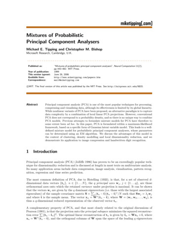
Mixtures of Probabilistic Principal Component Analyserswhere A T (A 1 )T . Thus if WML and ΨML are maximum likelihood solutions for the originaldata, then AWML and AΨML AT will be maximum likelihood solutions for the transformed dataset.In general the form of the solution will not be preserved under such a transformation. However,we can consider two special cases. First, suppose Ψ is a diagonal matrix, corresponding to thecase of factor analysis. Then Ψ will remain diagonal provided A is also a diagonal matrix. Thissays that factor analysis is covariant under component-wise rescaling of the data variables: thescale factors simply become absorbed into rescaling of the noise variances, and the rows of Ware rescaled by the same factors. Second, consider the case Ψ σ 2 I, corresponding to PPCA.Then the transformed noise covariance σ 2 AAT will only be proportional to the unit matrix ifAT A 1 , in other words if A is an orthogonal matrix. Transformation of the data vectorsby multiplication with an orthogonal matrix corresponds to a rotation of the coordinate system.This same covariance property is shared by standard non-probabilistic PCA since a rotation ofthe coordinates induces a corresponding rotation of the principal axes. Thus we see that factoranalysis is covariant under component-wise rescaling, while PPCA and PCA are covariant underrotations, as illustrated in Figure 1.Figure 1: Factor analysis is covariant under a component-wise rescaling of the data variables(top plots) while PCA and probabilistic PCA are covariant under rotations of thedata space coordinates (bottom plots).4Mixtures of Probabilistic Principal ComponentAnalysersThe association of a probability model with PCA offers the tempting prospect of being able tomodel complex data structures with a combination of local PCA models through the mechanism8

Mixtures of Probabilistic Principal Component Analysers9of a mixture of probabilistic principal component analysers (Tipping and Bishop 1997). This formulation would permit all of the model parameters to be determined from maximum-likelihood,where both the appropriate partitioning of the data and the determination of the respective principal axes occur automatically as the likelihood is maximized. The log-likelihood of observing thedata set for such a mixture model is:L NXln {p(tn )} ,n 1 NXlnn 1(MX(19))πi p(tn i) ,(20)i 1wherePp(t i) is a single PPCA model and πi is the corresponding mixing proportion, with πi 0andπi 1. Note that a separate mean vector µi is now associated with each of the M mixturecomponents, along with the parameters Wi and σi2 . A related model has recently been exploitedfor data visualization (Bishop and Tipping 1998), while a similar approach, based on the standardfactor analysis diagonal (Ψ) noise model, has been employed for handwritten digit recognition(Hinton et al. 1997), although it does not implement PCA.The corresponding generative model for the mixture case now requires the random choice of amixture component according to the proportions πi , followed by sampling from the x and ² distributions and applying equation (2) as in the single model case, taking care to utilise the appropriate parameters µi , Wi and σi2 . Furthermore, for a given data point t, there is now aposterior distribution associated with each latent space, the mean of which for space i is given by(σi2 I WiT Wi ) 1 WiT (t µi ).We can develop an iterative EM algorithm for optimization of all of the model parameters πi , µi ,Wi and σi2 . If Rni p(i tn ) is the posterior responsibility of mixture i for generating data pointtn , given byp(tn i)πiRni ,(21)p(tn )then in Appendix C it is shown that we obtain the following parameter updates:N1 XRni ,N n 1PNRni tne i Pn 1.µNn 1 Rniπei (22)(23)e i correspond exactly to those of a standard Gaussian mixture formuThus the updates for πei and µlation (e.g. see Bishop 1995). Furthermore, in Appendix C, it is also shown that the combinationof the E- and M-steps leads to the intuitive result that the axes Wi and the noise variance σi2 aredetermined from the local responsibility-weighted covariance matrix:Si N1 Xe i )(tn µe i )T ,Rni (tn µπei N n 1(24)by standard eigen-decomposition in exactly the same manner as for a single PPCA model. However,as noted earlier in Section 3.4 (and also in Appendix A.5), for larger values of data dimensionalityd, computational advantages can be obtained if Wi and σi2 are updated iteratively according toan EM schedule. This is discussed for the mixture model in Appendix C.Iteration of equations (21), (22) and (23) in sequence followed by computation of Wi and σi2 , eitherfrom equation (24) using (14) and (15) or using the iterative updates in Appendix C, is guaranteedto find a local maximum of the log-likelihood (19). At convergence of the algorithm each weightmatrix Wi spans the principal subspace of its respective Si .

Mixtures of Probabilistic Principal Component Analysers10In the next section we consider applications of this PPCA mixture model, beginning with datacompression and reconstruction tasks. We then consider general density modelling in Section 6.5Local Linear Dimensionality ReductionIn this section we begin by giving an illustration of the application of the PPCA mixture algorithmto a synthetic data set. More realistic examples are then considered, with an emphasis on casesin which a principal component approach is motivated by the objective of deriving a reduceddimensionality representation of the data which can be reconstructed with minimum error. Wewill therefore contrast the clustering mechanism in the PPCA mixture model with that of a hardclustering approach based explicitly on reconstruction error as utilised in a typical algorithm.5.1Illustration for Synthetic DataFor a demonstration of the mixture of PPCA algorithm, we generated a synthetic dataset comprising 500 data points sampled uniformly over the surface of a hemisphere, with additive Gaussiannoise. Figure 2(a) shows this data.A mixture of 12 probabilistic principal component analysers was then fitted to the data using theEM algorithm outlined in the previous section, with latent space dimensionality q 2. Becauseof the probabilistic formalism, a generative model of the data is defined and we emphasise this byplotting a second set of 500 data points, obtained by sampling from the fitted generative model.These data points are shown in Figure 2(b). Histograms of the distances of all the data pointsfrom the hemisphere are also given to indicate more clearly the accuracy of the model in capturingthe structure of the underlying generator.5.2Clustering MechanismsGenerating a local PCA model of the form illustrated above is often prompted by the ultimategoal of accurate data reconstruction. Indeed, this has motivated Kambhatla and Leen (1997)and Hinton et al. (1997) to utilise squared reconstruction error as the clustering criterion in thepartitioning phase. Dony and Haykin (1995) adopt a similar approach to image compression,although their model has no set of independent ‘mean’ parameters µi . Using the reconstructioncriterion, a data point is assigned to the component that reconstructs it with lowest error, and theprincipal axes are then re-estimated within each cluster. For the mixture of PPCA model, however,data points are assigned to mixture components (in a soft fashion) according to the responsibilityRni of the mixture component for its generation. Since, Rni p(tn i)πi /p(tn ) and p(tn ) is constantfor all

Mixtures of Probabilistic Principal Component Analysers 3 propose that the responsibility of the jth analyser for reconstructing data point tn be given by rnj exp(¡E2 j 2¾2) nP j0 exp(¡E 2 j0 2¾ 2) o, where Ej is the corresponding reconstruction cost. This allows the model to be determined by the maximization of a pseudo-likelihood function, and