Transcription
Hindawi Publishing CorporationMathematical Problems in EngineeringVolume 2012, Article ID 912603, 20 pagesdoi:10.1155/2012/912603Research ArticleTowards Online Model PredictiveControl on a Programmable Logic Controller:Practical ConsiderationsBart Huyck,1, 2, 3 Hans Joachim Ferreau,3Moritz Diehl,3 Jos De Brabanter,1, 3 Jan F. M. Van Impe,2Bart De Moor,3 and Filip Logist21Department of Industrial Engineering, KAHO Sint-Lieven, Gebroeders De Smetstraat 1,9000 Gent, Belgium2BioTeC, Department of Chemical Engineering (CIT), KU Leuven, W. de Croylaan 46,3001 Leuven, Belgium3SCD, Department of Electrical Engineering (ESAT), KU Leuven, Kasteelpark Arenberg 10,3001 Leuven, BelgiumCorrespondence should be addressed to Jan F. M. Van Impe, jan.vanimpe@cit.kuleuven.beReceived 10 July 2012; Revised 1 October 2012; Accepted 1 October 2012Academic Editor: Wei-Chiang HongCopyright q 2012 Bart Huyck et al. This is an open access article distributed under the CreativeCommons Attribution License, which permits unrestricted use, distribution, and reproduction inany medium, provided the original work is properly cited.Given the growing computational power of embedded controllers, the use of model predictive control MPC strategies on this type of devices becomes more and more attractive. This paper investigates the use of online MPC, in which at each step, an optimization problem is solved, on both aprogrammable automation controller PAC and a programmable logic controller PLC . Threedifferent optimization routines to solve the quadratic program were investigated with respectto their applicability on these devices. To this end, an air heating setup was built and selected as asmall-scale multi-input single-output system. It turns out that the code generator CVXGEN is notsuited for the PLC as the required programming language is not available and the programmingconcept with preallocated memory consumes too much memory. The Hildreth and qpOASES algorithms successfully controlled the setup running on the PLC hardware. Both algorithms performsimilarly, although it takes more time to calculate a solution for qpOASES. However, if the problemsize increases, it is expected that the high number of required iterations when the constraints arehit will cause the Hildreth algorithm to exceed the necessary time to present a solution. For thissmall heating problem under test, the Hildreth algorithm is selected as most useful on a PLC.1. IntroductionModel predictive control MPC has become a widely applied control technique in processindustry for the control of large-scale installations, which are typically described by
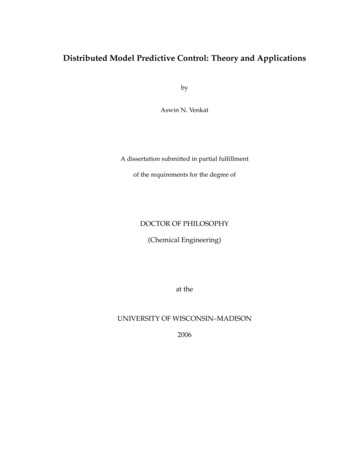
2Mathematical Problems in Engineeringlarge-scale models with relatively slow dynamics 1, 2 . The key element in MPC is to repeatedly solve an optimization problem based on available measurements of the current stateof the process. The advantages of MPC over classic PID control are its ability i to steer theprocess in an optimal way while taking proactively desired future behaviour into account, ii to tackle multiple inputs and outputs simultaneously, and iii to incorporate constraints 3 .In most cases, the MPC controller is hosted by a computer and employed as a supervisorycontroller, controlling the set-points of controllers closer to the process, for example, PIDs.In the recent years, interest has grown to exploit MPC on embedded systems. Typicalapplications are, for example, mechatronic systems, which give rise to small-scale modelswith fast dynamics 4–6 . In these cases the MPC controller is not a supervisory controlleranymore but directly steers the actuators and as such also the process itself.Compared to a standard PC, which nowadays has several cores with speeds in theGHz range and several GBs of memory, embedded controllers are typically implemented ondevices with much less computation power and memory. As indicated in Figure 1, a variety ofdevices exist. Programmable logic controllers PLCs are often exploited in industry for controltasks because of their robust operation, even in harsh conditions. They typically have a processing power in the order of only MHz and memory in the range from a few kB to severalMBs. Programmable automation controllers PACs bridge the gap as they exhibit a processingpower and memory that can go up to that found in PCs, combined with the I/O possibilitiesof a PLC. Hence, they can be employed to robustly fulfill also other tasks than control e.g.,data logging and maintaining network connections , as they can easily be integrated viastandard communication protocols.To deal with the computational limitations of embedded hardware, two approachescan be taken when implementing MPC on embedded hardware: explicit and online MPC.Explicit MPC 7, 8 precomputes all sets of possible solutions to the underlying optimizationproblem offline and stores them in a look-up tree. When running the controller online, mainlythe right working set has to be selected each time. As this approach avoids the online solutionof an optimization problem, high-speed algorithms are obtained for small-scale systems e.g.,single-input single-output SISO systems , with short prediction horizons. However, forlarger systems e.g., multiple-input multiple-output MIMO systems the number of working sets quickly grows and the time to search the look-up tree becomes prohibitive. In thesecases, online MPC, which exploits tailored algorithms for the online solution of the optimization problem 9 , becomes attractive.A prerequisite in industry is the use of reliable, easy-to-maintain control hardware,explaining the current dominance of PLCs today. Historically, PLC programming languageshave focused on the relay ladder logic RLL . Although more PC-like programming languages exist in the international standard IEC 61131-3, PLC programmers still more often useladder languages 10 . As a result, MPC implementations on PLCs are scarce see, e.g., 11, 12 for explicit MPC .The aim of the current paper is to illustrate the practical feasibility of online MPC withconstraints on PLCs. To this end, a test strategy is followed which exploits different types ofcontrol hardware with decreasing computation power. First, a PAC CompactRIO, NationalInstruments is used, and afterwards a PLC S7-319, Siemens is employed. Differentapproaches for solving the optimization problem are evaluated on a test setup. This onlineoptimization problem boils down to the solution of a quadratic program QP . The performance of three QP solvers will be compared when implemented on a PAC and a PLC. The firstalgorithm is the Hildreth QP algorithm 13 , a classic but easy to implement algorithm witha limited number of code lines. It will be compared to qpOASES, a state-of-the-art online
Mathematical Problems in re 1: Graphical comparison where to situate PLC, PAC, and PC to each other in view of speed andmemory.active set algorithm 14 that is provided in C/C . The third QP solver is CVXGEN, a Ccode generator for QP-representable convex optimization problems. The practical test setupinvolves a heating device where fan speed and resistor power can be manipulated independently to control the air temperature. As such, this device can be regarded as a multiple-inputsingle-output system. Although, small scale, it is an interesting application for testing, whichhas also been used by, for example, 11 . The observations allow the formulation of practicalguidelines and warnings for possible pitfalls.This paper is structured as follows Section 2 briefly repeats the MPC formulation andthe steps required to obtain a linear system model. Section 3 describes the practical implementation of the controller and the QP solvers used. A description of the experimental setup canbe found in Section 4. Section 5 contains the results for the model identification as well as forthe control of the setup using the PAC and the PLC. Finally, the main conclusions are summarized in Section 6.2. Steps towards Online MPC ImplementationFirst of all, the model predictive control needs a process model. For the design of the controller, several decisions need to be taken, for example the length of the different horizons, theselection of input, state or output constraints. Once these decisions have been made, the controller can be implemented and tested.2.1. Modelling the ProcessThere are several ways to obtain a model for control. Based on the physical and chemical lawsunderlying the process, a white-box model can be deduced. This modeling procedure is often
4Mathematical Problems in Engineeringtime intensive and, hence, expensive for large and complex systems. As time is money inindustry, faster ways are often preferred. Alternatively, available process data can be used tofit a black-box model based on generic mathematical relations. There are different black-boxmodelling techniques, linear 15–17 as well as nonlinear 18, 19 . In this paper, an MPC controller will be used that exploit a linear state space model constructed based on black-boxtechniques.2.2. Model Predictive Control FormulationLinear model predictive control is well known in the literature 3, 20, 21 , and the reader isinvited to read these works for a detailed description. The basic formulation is briefly givenbelow.A linear, time-invariant discrete-time system is described by:x k 1 y k Ax k Bu k , 2.1 Cx k ,with A Rn n , B Rn m , and C Rp n . Here m, n, and p are the number of inputs, states, andoutputs, respectively. The objective of the controller is to find the optimal input for this systemby means of minimizing a cost function:JHp i 1y k i k yref k i k 2Wy Hc 1 j 0 Δu k j k 2 .Wu 2.2 yref is the output reference and y is the predicted output. The formulation y k i k represents the vector y on sample time k i at calculation time k. The change of the input isΔu k j k u k j k u k j 1 k . Hp and Hc with Hc Hp are, respectively, theprediction and control horizon of the controller. Wy Rp p and Wu Rm m are positivedefinite weighting matrices.One of the key elements of MPC is the possibility to handle constraints. For this paperonly input constraints are taken into account: u j uMax , u j uMin . 2.3 Output and state constraints are omitted in the current study but can easily be introduced.The optimization problem can be formulated as the minimization of 2.2 , subject to 2.1 and 2.3 . In order to solve this problem, the optimization problem is reformulated by eliminationof the states in the form of a QP:min Jθ1 Tθ Hθ g T θ,2subject to : P θ α, 2.4 2.5
Mathematical Problems in Engineering5with 2.4 the quadratic objective function, 2.5 the linear inequalities constraints, and θ thedecision variables. To reformulate the problem, following steps are taken. First, the state spacemodel 2.1 is rewritten in terms of Δu and a new state x Δx,y 2.6 with Δx k x k x k 1 and y the current measured output 21 . The prediction over theprediction horizon is written in matrix formulation and is formulated as YFx QΔU, 2.7 with Y and ΔU column matrices of predicted outputs and delta inputs, respectively. Forexample, ΔU RnHc 1 composed of Δu k k to Δu k Hc 1 k . The matrices F and Qcan be found in many works on MPC 3, 21 . The matrix Q is postprocessed by including theweight matrices as follows:QT Wybd Q Wubd ,S 2.8 with Wybd and Wubd block diagonal matrices of Wy and Wu , respectively. As for the purpose ofthis work, the aim is to minimize the online calculation work; matrices that can be computedin advance are calculated offline. Matrix S is one of the precomputed matrices that does notchange during runtime. Vector g from 2.4 has to be calculated online. It contains two partsdepending on the current state and the reference of the in- and outputs. So, g has to be calculated according toG1 x G2 Yref ,g 2.9 where G1 and G2 are gradient matrices. Yref is an RpHc 1 matrix of the references yref k k toyref k Hp k . The gradient matrices are constant and are computed offline:G1ST WyTbd F,G2ST WyTbd . 2.10 The constraints, that is, the minimum and maximum admissible values for ΔU, are calculatedonline. ΔUMax is a column matrix of Hc times ΔuMax uMax u k 1 . ΔUMin is a columnmatrix of Hc times ΔuMin uMin u k 1 . Finally, the QP problem to be solved is1ΔUT SΔU gΔU,2subject to : ΔUMin ΔU ΔUMax ,g G1 x G2 Yref .minΔU 2.11 The Hildreth algorithm 13 , qpOASES 14 , and CVXGEN 22 will be used to solve this QPproblem.
6Mathematical Problems in Engineering2.3. Implementation of the MPC ControllerWhen the model is known and all parameters in the cost function are fixed, the controllercan be simulated and implemented. The hardware determines the speed of calculation andrestricts the size of the problem. Certainly in an embedded environment, this is an importantfactor. The following section deals with these problems when aiming for online MPC on aPLC.3. The ApproachWhen the process model has been identified, it is possible to simulate the process and tunethe controller to find valid and useful settings. Going towards online MPC on a PLC meansthat we have to deal with a shrinking amount of memory and a decreasing CPU speed. Tothis end, the MPC algorithm is analysed and parts that remain unchanged during runtime areprecomputed and lifted out of the online calculations. The limited amount of memory limitsthe size of the problem.3.1. The HardwareFor the practical implementation, two different controllers are used. First, a NationalInstruments CompactRIO is used. This PAC controller consists of a NI cRio–9024 Real-TimeController 800 MHz CPU, 512 Mb memory , a cRIO–9114 Reconfigurable Chassis, an NI 9265Analogue Current Output module, and an NI 9217 RTD 24-Bit Analogue Input Module. ThisReal-Time controller is programmed with LabVIEW and is able to run a software librarycompiled from C/C code via a call library function. The library is compiled for the VxWorks6.3 operating system with the gcc-compiler version 3.4.4. Second, a Siemens CPU3193DP/PN PLC is used. The base memory of this CPU is increased to the maximum allowed8 Mb. This CPU is the fastest S7-300 CPU. It takes 40 ns for one floating-point operation. Anadditional SM334 analogue card is employed to connect to the solid-state relays and DCdrive. The Siemens CPU is programmed using the Step 7 Professional 2010 software. To codethe problem, the structured control language S7-SCL is used. This programming languagecorresponds to STL in the standard IEC 61131-3.3.2. Practical ImplementationTo compute a new input for the process, the following sequence of actions, presentedin Algorithm 1 are implemented. In advance, constant matrices are precomputed and thereference trajectory for the output is selected.3.2.1. Programming the PACThe CompactRIO is running VxWorks as its operating system. A compiler exists to convertC/C code. All implemented QP solvers are originally written in C or C and are converted into a library. The preparative calculations, for instance, the scaling of the in- and outputs,the estimation of the state, and the selection of the current reference, are programmed inLabVIEW.
Mathematical Problems in Engineering7Offline: Calculate H’, G1 and G2Online: Start PLC or PACStore all precomputed matrices in working memory, together with the reference forinputs and outputwhile CPU is running doif 1 second passed since last call thenScale the temperaturesCalculate current state Calculate g, Umin and Umaxcase Hildreth algorithmCalculate the unconstrained inputs of the process.if unconstrained inputs violate constraints thenwhile maximum numbers of iterations is not reached and solution notfound doSolve one iteration of the QPendif maximum numbers of iterations is reached thenUse unconstrained solution with inputs violating the constraintlimited to the constraintendendendswcase qpOASESwhile maximum numbers of iterations is not reached and solution notfound doSolve one iteration of the QPendif maximum numbers of iterations is reached thenUse last sub-optimal solutionendendswcase CVXGENwhile maximum numbers of iterations is not reached and solution notfound doSolve one iteration of the QPendif maximum numbers of iterations is reached thenUse unconstrained solution with inputs violating the constraint limitedto the constraintendendswApply the inputs to the systemendendAlgorithm 1: Steps to compute the inputs of the experimental set-up.3.2.2. Programming the PLCThere exists no compiler to transform the C/C source code to a running binary on aSiemens PLC. Therefore, the C/C code has to be translated into S7-SCL STL . Althoughpossible, this is a time consuming step. In this project, the qpOASES and hildreth solvers aretranslated to S7-SCL. The qpOASES solver is translated without the hotstarting possibilities
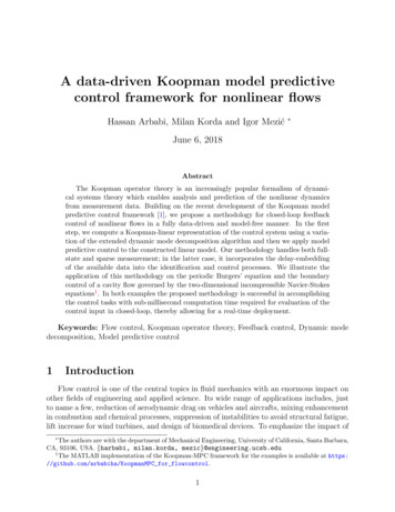
8Mathematical Problems in EngineeringOB100 OB10OB35OB1OB11OB35OB1OB12t (s)Figure 2: Schematic overview of the different organization blocks in the PLC.and the general constraint handling code. Instead, only the part that handles bounds is translated. CVXGEN cannot generate STL code, and a manual translation of the generated codeis impossible, hence; it is not used.To calculate the appropriate inputs of the system and solve the QP, following built-infunction blocks FBs and organization blocks OBs are programmed. Organization blocksare built-in functions called by hardware interrupts. Function blocks are user defined functions with corresponding data stored in a data block DB with the same number. Figure 2depicts the order in which these blocks are called.B 100: Cold StartThis block is called once when the controller is started. It calls function FB 1, which is usedto initialize the precomputed matrices larger than the 256 elements which are stored in DB2 linked to FB 2. This procedure is followed to overcome the limitation that an array ofconstants cannot be larger the 256 elements at compilation time. In the case a matrix needsto contain more than 256 elements, more arrays are combined in this block at runtime into acombined array. For these experiments, only matrix G2 is initialized in this function.OB 1: Main LoopThis loop is started as soon as OB 100 is finished. When this function finishes, it restarts again.This loop is used to program standard tasks of the PLC. In this experiment, it is not used. Itwill run during the idle time of the CPU between two OB35 calls.OB 35: Timed LoopThis organization block is called every second. It contains the necessary code to read thecurrent inputs. This information is scaled and employed to calculate the current state FB 3 .Together with the reference for the in- and outputs, the state is used to update vector g FB 2 .Now, the QP is solved and the scaled solution will be passed to the outputs of the PLC.3.3. A Solution to the QP: Algorithms3.3.1. The Hildreth AlgorithmThe Hildreth algorithm has been chosen for its limited number of code lines which makesit easy to implement. It has been written in C for the PAC and in S7-SCL for the PLC. Thisalgorithm calculates the solution in two steps 21 . First, the unconstrained solution is calculated, and if no constraints are violated, this solution is adopted. If a constraint is violated,a constrained QP is solved. The solution of the QP is then passed to the inputs of the heating
Mathematical Problems in Engineering9device. For more information about the solution routing, see 13, 21, 23 . If a solution tothe QP could not be found, the unconstrained solution is compared to the constraint. If aconstraint is violated, that entry of the unconstraint solution is limited to the constraint.3.3.2. qpOASESqpOASES is an open-source C implementation of the recently proposed online active setstrategy 14 . It builds on the idea that the optimal sets of active constraints do not differ muchfrom one QP to the next. At each sampling instant, it starts from the optimal solution of theprevious QP and follows a homotopy path towards the solution of the current QP. Along thispath, constraints may become active or inactive as in any active set QP solver and the internalmatrix factorizations are adapted accordingly. While moving along the homotopy path, theonline active set strategy delivers sub-optimal solutions in a transparent way. Therefore, suchsuboptimal feedback can be reasonably passed to the process in case the maximum numberof iterations is reached.A simplified version of qpOASES has been translated to S7-SCL and was used forcontrolling the heating device. Note that our simplified implementation does not allow forhot starting the QP solution and is not fully optimized for speed. Moreover, it only handlesbounds on the control inputs but no general constraints. On the PAC the plain ANSI C implementation of qpOASES has been used. Although the full version of qpOASES is perfectlysuited for hot starting, this is not used as the employed implementations of neither theHildreth algorithm nor the CVXGEN have possibilities to use hotstart. Moreover, based onthe knowledge that a solution is found in one step if no constraints are active, the algorithm isonly used with cold starts. This makes it possible to start the search for a solution with offlinecomputed matrices. On the other hand, qpOASES will most probably benefit from hotstartingif constraints are active as the number of required iterations decreases.3.3.3. CVXGENAccording to the website http://www.cvxgen.com/ , CVXGEN 22 generates fast customcode for small, QP-representable convex optimization problems, using an online interfacewith no software installation. With minimal effort, a mathematical problem description can beturned into a high speed solver. The generated code is C-code that should run on any devicesupporting this programming language. It works best for small problems, where the finalKKT-matrix has up to 4000 nonzero matrix entries. CVXGEN does not work well for largerproblems. The mathematical representation of the QP problem is presented to the webinterface and the generated code is compiled for the VxWorks operating system of theCompactRIO. Similar to the Hildreth algorithm, the unconstrained solution, limited to theconstraints when violated, is employed if a solution to the QP cannot be found.4. Experimental SetupThe temperature control setup Figure 3 consists of a resistor and a fan which can be manipulated separately. The fan is driven by a 24 V DC motor, and the resistor has a maximumpower of 1400 W. The heating power delivered by the resistor can be adapted by solid-staterelays with analog control Gefran GTT 25 A 480 VAC—analogue control voltage 0–10 V .
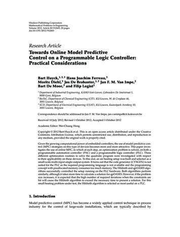
10Mathematical Problems in re 3: Schematic overview of the temperature control setup.The fan is manipulated by a custom made DC drive based on a Texas Instruments DRV102Tchip and adapted for an analogue control voltage of 0–10 V. Temperature sensors measure theenvironmental temperature and the temperature of the heated air as indicated in Figure 3.Both sensors are of the PT100 class B type.5. Results5.1. Model IdentificationTo control the experimental setup, a two-input fan speed and resistor power and singleoutput temperature black-box model is constructed with the Matlab System IdentificationToolbox 24 . A linear, low-order, continuous-time transfer function of the formG s Kpe Td s .1 Tp1 s 5.1 is fitted to the data and named P1D. Afterwards, this model is discretized and converted tostatespace of the form 2.1 . This model is called P1DSS. The excitation signal of the identification experiment is a multisine with frequencies within the range 0.05–0.00125 Hz. Afterdetrending and normalization, this dataset, is divided in an estimation and validation setwith each a length of 250 s. To determine the model quality, a fit measure is defined over thevalidation data: Y Y 2 100% 1 , Y Y fit 5.2 2where Y is the simulated output, Y the measured output, and Y the mean of the measuredoutput. A fit value of 100% means that the simulation is the same as the measured output.The final identified P1D model is Tn 0.98 1.34s 0.83ee 1.53s1 5.17s1 7.17s uFan,n,uPower,n 5.3
Mathematical Problems in Engineering116560Temperature ( C)55504540353025050100150200250Time (s)P1D (79.5%)Measured temperatureFigure 4: Validation of the P1D model on multisine validation data.where the index n indicates a normalised variable. uFan,n and uPower,n are, respectively, thenormalized and detrended actuator voltage for the motor drive and the solid state relays ofthe resistor. After detrending, a zero output of the model corresponds to 42 C. For the inputs,the zero input corresponds to 5 V. Conversion to state space of the P1D model with a discretisation interval of 1 s, results in a discrete state space model of order 4. This model is controllable, observable, and stable. The validation of the P1D model is depicted in Figure 4. Thefit is 79% for both the P1D and P1DSS model.5.2. Controller DesignThe P1DSS model is selected as controller model. The control horizon Hc of the controller isset to 7 and the prediction horizon Hp is 22. These horizons have been chosen similar to thosein 25 , to compare the different controllers and control algorithms for this temperaturecontrol setup. These horizons turned out to be the maximum settings if an MPC controller isbuilt with CVXGEN for use on the PAC.5.3. Controlling the SetupOn each controller device, three experiments, each time with a different QP algorithm, areexecuted. The weight matrix Wu in the cost function is the identity matrix:WuI2 2 1 0.0 1 5.4 Wy is set to one. Each experiment consists of a reference trajectory for the temperature of10 minutes. This reference is first at a constant temperature of 40 C during 100 s. To ensure
12Mathematical Problems in Engineeringthat the data logging program is ready and the estimator has reached a steady-state valueon both PAC and PLC, the inputs calculated by the controller are only applied from 30 s on.During the first 30 s, the fan speed is set to 20% of its maximum speed and the resistor poweris 0. After 100 s, the setpoint jumps to 45 C and 60 C for 60 s each. This stair is followed by ahalf period of a cosine that should bring the temperature at 20 C. This is below the environmental temperature of approximately 22 C and therefore unreachable. This part of thetrajectory is added to make sure the controller hits the constraints for a number of seconds.From 320 s on, the temperature reference is set to 30 C for 60 s, followed by a ramp of 30 s witha slope 0.1 C/s. At the end of the ramp there is a jump towards 50 C. This temperature is keptconstant for 60 seconds and followed by another set-point change to 30 C for 60 seconds. Toend the experiment the temperature is fixed at 40 C. It has to be noted that all algorithmsand implementations have tested beforehand in simulation. In this case identical results havebeen obtained as the solution to the QP is unique. The simulations have been executed inMatlab and LabVIEW. The latter are hardware-in-the-loop simulations. Thereto we have usedthe code and libraries also used for the experiments on the real setup, but instead of the realsetup, a linear model is used.5.3.1. MPC on a PACAll three QP algorithms are tested on the CompactRIO PAC system. Figure 5 depicts the controlled temperature along the reference and the corresponding inputs.The Resulting Temperature ControlThe controlled temperature follows the reference accurately when all transient effects havefaded. The incorporated integrator eliminates the steady-state error. The plots show oscillating behaviour at steps when the reference is above 45 C. This is explained by the limitedvalidity of the linear model at these temperatures. This oscillation behavior is unwanted andhas to be corrected with different controller settings, for example, an increasing Wu . In orderto make a fair comparison with the PLC experiments these settings are not changed. All threealgorithms start the experiment with a large overshoot. It is caused by the large step from theenvironmental temperature to 40 C and the mismatch between the estimated state from thelinear model and the real system. For the next step around 80 seconds, an overshoot is hardlyseen. The mismatch between the model and the real heating setup is small at this point. Thenext jump towards 60 C is outside the validity region of the model and this is clearly seen asan overshoot followed by oscillations. The cosine function is followed accurately, except at theend, where the set-point is below the environmental temperature. This makes it impossibleto track the desired temperature. After 300 s, the set-point evolves slowly to 30 C as both constraints are active. The next ramp is followed with a delay of one to two seconds. At the endof the ramp, the 10 C jump causes again a large overshoot as the mismatch between the modeland real system is large at 50 C. The transition to 30 C leads to a small nonoscillating undershoot.Important to notice is that all three algorithms behave almost identically. The meansquared-error MSE values are calculated and differ by at most 3%. The small differencesin the output Figure 5 a and inputs Figure 5 b are caused by different environmentalconditions. An open window is responsible for a soft breeze in the room from time to time.
Mathematical Problems in Engineering137060Temperature ( C)50403020100100200300400500600Time (s)qpOASES Wu11Hildreth Wu11CVX Wu11Reference a Measured temperature. The controlled output of the systemHeating (V)864200100200300400500600400500600Fan speed (V)Time (s)87654320100200300Time (s)qpOASES Wu11Hildreth Wu11CVX Wu11 b The applied inputs to the systemFigure 5: The in- and outputs for the Hildret
Programmable logic controllers PLCs are often exploited in industry for control tasks because of their robust operation, even in harsh conditions. They typically have a pro-cessing power in the order of only MHz and memory in the range from a few kB to several MBs. Programmable automation controllers PACs bridge the gap as they exhibit a processing