Transcription
Study MaterialCourse No.: Ag Econ 122(Production Economics and Farm Management)Credit Hours:1 1 2;Semester:IIPrepared byVirender KumarProfessor (Agricultural Economics)Department of Agricultural Economics, Extension Education & Rural Sociology, COA,CSKHPAU, Palampur-176 062 (HP), IndiaCourse Contents (Theory) Production Economics: Meaning, definition. Nature and scope of Agricultural Production Economics. Basic concepts and terms. Meaning and types of production functions Laws of returns: Increasing, constant and decreasing. Factor-product relationship. Determination of optimum input and output. Factor-factor relationship. Product-product relationship. Type of enterprise relationship. Returns to scale: meaning, definition, importance. Farm management definition, scope, importance. Typical farm management decisions. Economic principles applied to the organization of farm business. Types and systems of farming, Cost concepts and farm efficiency. Farm planning and budgeting. Risk and uncertainty. Linear programming: Assumption, advantages and limitations of linear programming.
Course Outline (Practical) Application of Farm Management Principles Computation of cost concepts Methods of consumption of depreciation Analyses of net worth statement Farm inventory analysis Preparation of farm plans and budgets Types of farm records and account Preparation of profit and loss account Break even analysis Cost of cultivation and economic analysis of different crop and livestock enterprises.Examination Schedule & Distribution of Marks:1.Mid Term Practical (Internal)15%2End Term Practical (Internal)35%3End Term Theory (External)50%Total Marks100References1. Johl, S.S. and Kapoor, T.R. (1973), Fundamentals of Farm Business Management,Kalyani Publishers, Ludhiana.2. Sankhayan, P.L. (1988), Introduction to the Economics of Agricultural Production,Prentice Hall of India Private Limited, New Delhi-110 001.3. Raju, V.T. and Rao, D.V.S. (1990), Economics of Farm Production and Management,Oxford & IBH Publishing Co. Pvt. Ltd., New Delhi-110 001.4. Dhondyal, S.P. (1985), Farm Management, Friends Publication Meerut (India).5. Kahlon, A.S. and Karam Singh (1992), Economics of Farm Management, AlliedPublishers, New Delhi.6. Doll, John P. and Orazem. F. (1984), Production Economics: Theory with Application,John Wiley and Sons, New York.
Lecture 1Production Economics-Meaning & Definition, Nature andScope of Agricultural Production EconomicsAgricultural EconomicsAs a separate discipline, agricultural economics started only in the beginning of 20thcentury when economic issues pertaining to agriculture aroused interest at severaleducational centres. The depression of 1890s that wrecked havoc in agriculture at manyplaces forced organized farmers groups to take keen interest in farm managementproblems. The study and teaching of agricultural economics was started at HarvardUniversity (USA) in 1903 by Professor Thomas Nixon Carver. Agricultural economicsmay be defined as the application of principles and methods of economics to study theproblems of agriculture to get maximum output and profits from the use of resources thatare limited for the well being of the society in general and farming industry in particular.Nature and Scope of Agricultural EconomicsAgriculture sector has undergone a sea change over time from being subsistence innature in early stages to the present day online high-tech agribusiness. It is no moreconfined to production at the farm level. The storage, processing and distribution ofagricultural products involve an array of agribusiness industries. Initially, agriculturaleconomics studied the cost and returns for farm enterprises and emphasized the study ofmanagement problems on farms. But now it encompasses a host of activities related tofarm management, agricultural marketing, agricultural finance and accounting,agricultural trade and laws, contract farming, etc.Both microeconomics and macroeconomics have applications in agriculture. Theproduction problems on individual farms are important. But agriculture is notindependent of other sectors of the economy. The logic of economics is at the core ofagricultural economics but it is not the whole of agricultural economics. To effectivelyapply economic principles to agriculture, the economist must understand the biologicalnature of agricultural production. Thus, agricultural economics involves the unique blend
of abstract logic of economics with the practical management problems of modern dayagriculture.The widely accepted goal of agricultural economics is to increase efficiency inagriculture. This means to produce the needed food, fodder, fuel and fibre withoutwasting resources. To meet this goal, the required output must be produced with thesmallest amount of scarce resources, or maximum possible output must be obtained froma given amount of resources.Definition: Production economics is the application of the principles of microeconomicsin production.Based on the theory of firm, these principles explain various costconcepts, output response to inputs and the use of inputs/resources to maximize profitsand/ or minimize costs. Production economics, thus provides a framework for decisionmaking at the level of a firm for increasing efficiency and profits.Why study production processThe study of production economics is important in answering the following questions:1. What is efficient production?2. How is most profitable amount of inputs determined?3. How the production will respond to a change in the price of output?4. What enterprise combinations will maximize profits?5. What should a manager do when he is uncertain about yield response?6. How will technical change affect output?Agricultural Production EconomicsIt is a sub-discipline within the broad subject of agricultural economics and is concernedwith the selection of production patterns and resource use efficiency so as to optimize theobjective function of farming community or the nation within a framework of limitedresources. It may be defined as an applied field of science wherein principles ofeconomic choice are applied to the use of resources of land, labour, capital andmanagement in the farming industry.
Goals of Production EconomicsThe following are the goals of agricultural production economics:1. Assist farm managers in determining the best use of resources, given the changingneeds, values and goals of the society.2. Assist policy makers in determining the consequences of alternative publicpolicies on output, profits and resource use on farms.3. Evaluate the uses of theory of firm for improving farm management andunderstanding the behaviour of the farm as a profit maximizing entity.4. Evaluate the effects of technical and institutional changes on agriculturalproduction and resource use.5. Determine individual farm and aggregated regional farm adjustments in outputsupply and resource use to changes in economic variables in the economy.Subject Matter of Agricultural Production EconomicsAgricultural production economics involves analysis of production relationships andprinciples of rational decision making to optimize the use of farm resources on individualfarms as well as to rationalize the use of farm inputs from the point of view of the entireeconomy. The primary interest is in applying economic logic to problems that occur inagriculture. Agricultural production economics is concerned with the productivity of farminputs. As such it deals with resource allocation, resource combinations, resource useefficiency, resource management and resource administration. The subject matter ofagricultural production economics involves the study of factor-product, factor-factor andproduct-product relationships, the size of the farm, returns to scale, credit and risk anduncertainty, etc. Therefore, any problem of farmers that falls under the scope of resourceallocation and marginal productivity analysis is the subject matter of agriculturalproduction economics.Objectives1. To determine and outline the conditions that give the optimum use of capital,labour, land and management resources in the production of crops, livestock andallied enterprises.
2. To determine the extent to which the existing use of resources deviates from theoptimum use.3. To analyse the forces which condition the existing production pattern andresource use.4. To explain the means and methods in getting from the existing use to optimumuse of resources.
Lecture 2Agricultural Production Economics: Basic Concepts1. Production: The process through which some goods and services called inputs aretransformed into other goods called products or output.2. Production function: A systematic and mathematical expression of therelationship among various quantities of inputs or input services used in theproduction of a commodity and the corresponding quantities of output is called aproduction function.3. Continuous production function: This function arises for those inputs which canbe divided into smaller doses. Continuous variables can be known frommeasurement, for example, seeds and fertilizers, etc.4. Discontinuous or discrete production function: This function arises for thoseinputs or work units which cannot be divided into smaller units and hence areused in whole numbers. For example, number of ploughings, weedings andharvestings, etc.5. Short run production period: The planning period during which one or more ofthe resources are fixed while others are variable resources. The output can bevaried only by intensive use of fixed resources. It is written asY f (X1, X2 / X3 .Xn) where Y is output, X1, X2 are variableinputs and X3 .Xn are fixed inputs.6. Long run production period: The planning period during which all the resourcescan be varied. It is written asY f (X1, X2 , .Xn)7. Technical coefficient: The amount of input per unit of output is called technicalcoefficient.8. Resources: Anything that aids in production is called a resource. The resourcesphysically enter the production process.9. Resource services: The work done by a person, machine or livestock is called aresource service. Resources do not enter the production process physically.
10. Fixed resources: The resources that remain unchanged irrespective of the level ofproduction are called fixed resources. For example, land , building, machinery.These resources exist only in short run. The costs associated with these resourcesare called fixed costs.11. Variable resources: The resources that vary with the level of production arecalled variable resources. These resources exist both in short run and long run.For example, seeds, fertilizers, chemicals, etc. The costs associated with theseresources are called variable costs.12. Flow resources: The resources that cannot be stored and should be used as andwhen these are available. For example, services of a labourer on a particular day.13. Stock resources: The resources that can be stored for use later on. For example,seeds. Defining an input as a flow or stock depends on the length of time underconsideration. For example, tractor with 10 years life is a stock resources if wetake the services of tractor for its entire useful life of 10 years. But it alsoprovides its service every day, therefore it is a flow resources.14. Production period: It is the time period required for the transformation ofresources or inputs into products.15. Farm entrepreneur: Farm entrepreneur is the person who organizes and operatesthe farm business and bears the responsibility of the outcome of the business.16. Farm business manager: Person appointed by the entrepreneur to manage andsupervise the farm business and is paid for the services rendered. He/she carriesout the instructions of the entrepreneur.17. Productivity: Output per unit of inputs is called the productivity.18. Technical efficiency: It is the ratio of the physical output to inputs used. Itimplies the using of resources as effectively as possible without any wastages.19. Economic efficiency: It is the expression of technical efficiency in monetaryterms through the prices. In other words, the ratio of value of output to value ofinputs is termed as economic efficiency. It implies maximization of profits perunit of input.
20. izationofresources/production can make any combination higher yielding without makingother combination less yielding. It refers to resource use efficiency.21. Optimality: It is an ideal condition or situation in which costs are minimumand/or profits maximum.22. Cost of cultivation: The expenditure incurred on all inputs and input services inraising a crop on a unit area is called cost of cultivation. It is expressed as rupeesper hectare or rupees per acre.23. Cost of production: The expenditure incurred in producing a unit quantity ofoutput is known as cost of production, for example, Rs./kg of Rs./quintal.24. Independent variable: Variable whose value does not depend on other variablesand which influences the dependent variable, is termed as independent variable,for example, land, labour and capital.25. Dependent variable: Variable whose value depends on other variables is termedas dependent variable, for example, crop output.26. Slope of a line: It represents the rate of change in one variable that occurs whenanother variable changes. Slope varies at different points on a curve but remainssame on all points on a given line. It is the rate of change in the variable onvertical axis per unit change in the variable on horizontal axis and is expressed asa number.27. Total physical product: Total amount of output obtained by using different unitsof inputs measured in physical units, for example, kg, tonnes, etc.28. Average physical product (APP): Output per unit of input on an average is termedas APP and is given by Y/X.29. Marginal physical product: Addition to total output obtained by using themarginal unit of input and is measured as ΔY/ΔX.
Lecture 3Production Functions: Meaning and TypesThe production function portrays an input-output relationship. It describes the rate at whichresources are transformed into products. There are numerous input-output relationships inagriculture because the rates at which the inputs are transformed into outputs will vary amongsoil types, animals, technologies, rainfall amount and so forth.Definition: Production function is a technical and mathematical relationship describing themanner and extent to which a particular product depends upon the quantities of inputs or servicesof inputs, used at a given level of technology and in a given period of time. It shows the quantityof output that can be produced using different levels of inputs.A production function can be expressed in different ways: in written form, enumerating anddescribing the inputs that have a bearing on the output; by listing inputs and the resulting outputsnumerically in a table; depicting in the form of a graph or a diagram; and in the form of analgebraic equation. Symbolically, a production function can be written asY f (X1, X2 , X3 , ., Xn) where Y is output, X1, X2 , X3 . Xn are inputs. It,however, does not tell which inputs are fixed and which are the variable ones. Since inproduction, fixed inputs play an important role, these are expressed as: Y f (X1, X2 / X3 .Xn)where Y is output, X1, X2 are variable inputs and X3 .Xn are fixed inputs.Assumptions of Production Function Analysis1. The production function is defined only for the non-negative values of inputs and outputs.2. The production function presupposes technical efficiency. This means that every possiblecombination of inputs is assumed to result in maximum level of output.3. The input- output relationship or the production function is single valued and continuous.4. The production function is characterized by i) decreasing marginal product for all factorproduct combinations; ii) decreasing rate of technical substitution between any twofactors; and iii) an increasing rate of product transformation between any two products.5. The returns to scale are assumed to be decreasing.6. All the factors of production and products are perfectly divisible.7. The parameters determining the firm’s production function do not change over the time periodconsidered. Also, these parameters are not allowed to be random variables.
8. The exact nature of any production function is assumed to be determined by a set of technicaldecisions taken by the producer.Types of Production FunctionsSeveral types of production functions used in agriculture are as follows:i) Linear Production Function: Also known as first degree polynomial. It’s algebraic form isgiven byy a0 bxwhere a0 is the intercept and b is the slope of the function. It is not commonly used inresearch because it violates the basic assumptions of characteristic functional analysis.ii) Quadratic PF: Also known as second degree polynomial. This type of PF allows bothdeclining & negative marginal productivity thus embracing the second and third stage ofproduction simultaneously.y b0 b1 x1 b2 x12 where b0, b1 , & b2, are the parameters. Such PFs are quite common infertilizer response studies.iii) Cobb-Douglas PF: It is also known as power production function. It is most widely used PF.It accounts for only our stage of production at a time & cannot represent constant, increasing ordecreasing marginal productivity simultaneously.Y b0 x1b1where b0 is efficiency parameters & b1 is elasticity of productioniv) Mitscherlich or Spillman functionv) Transcendental functionvi) Translog PFvii) Constant elasticity of substitution (CES) functionviii) Resistance Functionix) Square root PF: It represents a compromise between C-D & the quadratic PF.
y a 0 a1x a2 xThis function gets rid of the limitations of field mix of inputs for producing different levels ofoutput inherent in the C-D production function & that of linear isoclines in quadratic function.Thus, this function allows both a diminishing TP in the same way as QF does & for decliningMPs at a diminishing rate as the C-D function does.
Lecture 4Laws of Returns: Increasing, Constant and DecreasingIn production one or a combination of the following relationships are commonlyobserved:1. Law of constant marginal returns (productivity),2. Law of increasing marginal returns (productivity) and3. Law of decreasing marginal returns (productivity)1. Law of constant marginal returns (productivity): It is said to operate when each marginalunit of variable input adds equal quantity of output to the total output. It is applicable overlimited range, e.g. one tractor (plus driver) will almost give same output, other things remainingconstant.Fertilizer (X)(in kg)01020304050Total Product (Y)(in kg)130013501400145015001550Marginal Product (Returns)(ΔY/Δ X)55555Algebraically, ΔY1/ΔX1 ΔY2/ΔX2 . ΔYn/ΔXn2. Law of increasing marginal returns (productivity): It is said to operate when each marginalunit of variable input adds more and more quantity of output to the total output. It is not commonin agriculture, e.g. small increase in seed input given the fixed inputs.Seed (X) (inkg)101520253035Total Product (Y)(in kg)100010251075115012501375Marginal Product (Returns)(ΔY/Δ X)510152025
Algebraically, ΔY1/ΔX1 ΔY2/ΔX2 . ΔYn/ΔXn3. Law of decreasing marginal returns (productivity): It is said to operate when eachmarginal unit of variable input adds less and less quantity of output to the total output. It iswidely applicable in agriculture.Fertilizer (X)(in kg)0102030405060Total Product (Y)(in kg)500140021002600300033003500Marginal Product (Returns)(ΔY/Δ X)907050403020Algebraically, ΔY1/ΔX1 ΔY2/ΔX2 . ΔYn/ΔXn
Lecture 5Factor-Product RelationshipDetermination of Optimum Input and OutputLaw of diminishing returns and the three stages of productionThe law of diminishing returns describes the relationship between output and the variable inputwhen other inputs are held constant.Definition: If increasing amounts of one input are added to a production process while all otherinputs are held constant, the amount of output added per unit of variable input will eventuallydecrease. It is also known as law of diminishing productivity or the law of variable proportions.Application of the law of diminishing returns to the production concept can result in a productionfunction of classical type. It displays increasing marginal returns first and then decreasingmarginal returns.The three stages of productionEp 1OutputYEp 0Ep 1TPPInflectionpointIIIIIIInput CongestionAPP0MPPXInput
Three stages of productionThe classical production function can be divided into three regions or stages, each beingimportant from the standpoint of efficient resources use.Stage-I occurs when marginal physical product (MPP) average physical product (APP). APPis increasing throughout this stage, indicating that the average rate at which X is transformed intoY, increases until APP reaches its maximum at the end of Stage-I.Stage-II occurs when MPP is decreasing and is less than APP but greater than zero. The physicalefficiency of the variable input reaches a peak at the beginning of Stage–II. On the other handphysical efficiency of fixed input is greatest at the end of Stage-II. This is because the number offixed input is constant and therefore the output/ unit of fixed input must be the largest when thetotal output from the production process is maximum.Stage-III occurs when MPP is negative. Stage III occurs when excessive quantities of variableinput are combined with the fixed input, so much, that total physical product (TPP) begins todecrease.Economic recommendations & production function analysis: Production function knowledgeand the input and output prices information can be used to know the most profitable input andoutput levels. However, even when price information is not available, some recommendationsabout the input use can be made from the production function itself.1.If the product has any value at all, input use once begun, should be continued until Stage–II is reached. That is because physical efficiency of variable resources, measured byAPP, increases throughout stage –I.2.Even if input is free, it will not be used in stage III. Maximum output occurs when StageII closes. It is of no use applying variable input when TPP starts coming down.3.Stage II defines the area of economic relevance. Variable input use must be somewherein stage-II, but exact input amount can be determined when choice indicators (input &output prices) are known.A. Relationship between TPP & MPP1. Since MPP is a measure of rate of change, therefore
(i) when TPP is increasing, MPP will be ve,(ii) when TPP is constant MPP will be zero,(iii) when TPP decreases, MPP will be –ve.2. So long MPP moves upward, TPP increases at an increasing rate.3. When MPP remains constant, TPP increases at a constant rate.4. When MPP starts declining, TPP increases at a decreasing rate.5. When MPP is zero, TPP will be at maximum.B. Relationship between MPP & APP1. When MPP is increasing, APP is also increasing. So long as MPP is above APP, the APPkeeps increasing.2. When MPP curve goes below APP curve, APP starts declining, that is, when AP is decreasingthe MP is always less than APP.3. When MP AP, AP will be at maximum. Here MP curve must intersect AP curve fromabove at its highest point.So whenMP APAP MP APAP MP APAP is at maximum.Elasticity of production: The elasticity of production is a concept that measures the degree ofresponsiveness between output and input. It is independent of the units of measurement.Ep % change in output% change in inputEp Y / Y Y / X MPP X / XY/XAPP
Ep 1 in Stage I0 Ep 1stage IIE p is negativestage IIIis based on exact MPPsThe point of diminishing returns can be defined to occur when MPP APP that is Ep 1 (lowerboundary of stage II) & this is the minimum amount of variable input that will be used & itoccurs when the efficiency of variable input is at its maximum. At the other end, MPP is zero,therefore Ep 0. Thus the relevant production zone is when O Ep 1.The optimum level of variable input is given by:ΔX1.PX1 ΔY. Py orΔY/ ΔX1. PX1/ PyMarginal cost marginal revenue.
Lecture 6Factor – Factor RelationshipFactor-factor relationship is concerned with the possibilities of substituting one input/factor (X1)for another input/factor (X2) for producing a given level of output. It answers the crucial questionof finding out the optimum or least cost combination of two or more resources in producing thegiven amount of output. The two fold object of factor-factor relationship is(i)Minimization of cost at a given level of output.(ii)Optimization of output to the fixed factors through alternatives resourcescombinations.The functional relationship is Y f (X1, X2/X3---Xn)what amounts of X1 & X2 should be used to give the lowest cost for producing fixed y0, when X3----- Xn areheld constant.Isoquant (Iso-product curve): It is defined as the locus of various combinations of two inputsyielding the same level of output. Each point on an isoquant represents the maximum output thatcan be attained with these input combinations. Isoquant is a convenient device for compressingthe 3-dimension picture of a production process into two dimensions. X1 f (X2, Y0).Isoquant mapX2X1Properties of isoquants1. Isoquants have a negative slope,
2.Isoquants to right indicate higher output level,3. Isoquants do not interest each other,4. Isoquant are convex to origin showing diminishing MRTS.Types of Factor-Factor Relationship: Many types of production surfaces are possibledepending upon the underlying production function. The shapes of the isoquants and productionsurfaces will depend on the manner in which the variable inputs are combined to produce aparticular level of output. Broadly, these are three categories of such combinations of inputs.(1) Fixed proportion combination of inputs,(2) Constant rate of substitution(3) Varying rates of substitution(1) Fixed proportion combinationThese represent such products that can be produced if inputs are added in fixed proportion at alllevels of production. In this case there is no substitution between inputs and thus there is strictcomplementarily between the two inputs. Such an isoquant implies that one exact combination ofinputs will produce a particular level of output. The inputs which increase the output only whencombined in a fixed proportion are known as complementary inputs, e.g. One tractor and oneman (driver). No problem in economic decision working. Also called Leontief isoquants.X2y3y2y1oX1Substitutes: Two resources are said to be substitutes when change in price of one leads to achange in demand for another (MRTS is –ve).
Complements: Resources used together in production. When Price of X1 increases the demandfor X2 decrease. (MRTS is zero).2. Constant rate of substitution: Such type of a factor-factor relationship gives linear isoquants.The substitution occurs at constant rate i.e. the amount of one input replaced by the other inputdoes not change as the added input increases. X 2 n X 21 X 22 ----------- X11 X 12 X 1nX2OX1Assumes perfect substitutbilityConstant SubstitutionX2Female labourX1Male labour X2ΔX1 X 2 MRTS X1 X1X 2 101212/1 282212/1 263212/1 244212/1 225212/1 2e.g. Two labourers. Decision rule use either of the two depending on the relative prices.3. Varying Rate of substitution: In this there can either be increasing rate or decreasing rate ofsubstitution. In this MRTSX1X2 varies over iso-product curve. It means that the amount of oneinput (X1) required to substitute for one unit of another input (X2) at a given level of production
increases or decreases as the amount of X1 used increases. Substitution at decreasing rate iscommon in agriculture (N& P or K & L) X 21 X 22 X 2 n -- -------- X 11 X 12 X 111X2Y10X1Fodder & concentratesThese convex isoquants represent continuous substitution between the two inputs. These are easyto handle mathematically (using calculus).MRTSX1X2 X 2 X 1
Marginal rate of technical substitution (MRTS or MRS): MRTS is defined as the negative ofthe slope of the isoquant at any point. It is the rate at which two factors of production can beexchanged at a particular level of output and consequently that of the levels of inputs used.Slope of isoquant MRTSX1X2 dy X 2 for (replaced ) MP1 X 1of (added )MP 2DyDy.dx1 .dX2DX 1DX 2dy 0 on an isoquantDydX 2DX 1 MP1 dX 1 DyMP 2DX 2Iso-cost line: Locus of all possible combination of two inputs which can be purchased with agiven outlay or budget.T PX1.X1 Px2.X2 or X1 ( TP x 2 (X 2 )P x1)P x1-X2X2X1X1
X2X2PX1 increase &PX2 DecreasesP X2 becomesCostlier &P X1 decreasesX1X1Two important points regarding iso-cost line are:(i)It prices are same and only outlay changes then iso-cost lines will be parallel to eachother.(ii)Changes in prices of inputs will change the slope of iso-cost line.Computing Least cost combination: Three methods(1) Arithmetical Method:Sr. X1No.X2output 85 unitsCost of X1@ Rs3.00/unitCost of X2 @ Rs4.00/unitTotal 3.5710.502838.5(2) Algebraic Method:MRSX1X2 X 2 X 1PX1 (ΔX1) PX2 (ΔX2)If PX1 (ΔX1) PX2 (ΔX2) Increase X2Price ratio PX 1PX 2
If PX1 (ΔX1) PX2 (ΔX2) Increase X1(3) Graphic Method:Slope of isoquant slope of iso-cost lineX2X02q1OX0 1X1Iso-cline: A line or curve connecting the least cost combinations of inputs for all output levels isknown as isocline. Isocline passes through all isoquants at points where they have same slope. Itshows how the relative proportion of the factors changes as the output is increased. It shows thatresources should be used along this line as long as MVP MC of resources used.Ridge lines: Represent the points of maximum output from each input, given a
and/ or minimize costs. Production economics, thus provides a framework for decision making at the level of a firm for increasing efficiency and profits. Why study production process The study of production economics is important in answering the following questions: 1. What is efficient production? 2. How is most profitable amount of inputs .