WIXLIB

STA561: Probabilistic machine learningKernels and Kernel Methods (10/09/13)Lecturer: Barbara Engelhardt1Scribes: Yue Dai, Li Lu, Will WuKernel Functions1.1What are Kernels?Kernels are a way to represent your data samples flexibly so that you can compare the samples in a complexspace. Kernels have shown great utility in comparing images of different sizes protein sequences of different lengths object 3D structures networks with different numbers of edges and/or nodes text documents of different lengths and formats.All of these objects have different numbers and types of features. We want to be able to cluster data samplesto find which pairs are neighbors in this complex, high dimensional space. A kernel is an arbitrary functionthat lets us map objects in this complex space to a high dimensional space that enables comparisons of thesecomplex features in a simple way. We have an X space of our samples, and a feature space that we defineby first defining a kernel function. This helps with:1. Comparing: it may be hard to compare two different text documents with different number of words.A properly-defined kernel gives us a metric by which we can quantify the similarities between twoobjects;2. Classification: even if we can quantify similarity in our feature space, simple classifiers may not performwell in this space. We may want to project our data to a different space and classify our samples inthis space.Previously in class, we used a fixed set of features and a probabilistic modeling approach. We turn to largemargin classifiers and a kernel-based approach in this lecture.1.2Kernel function.Given some abstract space X (e.g., documents, images, proteins, etc.), function κ : X X 7 R is called akernel function. Kernel functions are used to quantify similarity between a pair of objects x and x0 in X .1

2Kernels and Kernel MethodsA kernel function typically satisfies the following two properties (but this is not required for all kernelmethods). A kernel with these properties will loosely have the interpretation as a similarity quantificationbetween the two objects.(symmetric) x, x0 X , κ(x, x0 ) κ(x0 , x),(non-negative) x, x0 X , κ(x, x0 ) 0.1.3Mercer KernelsLet X {x1 , . . . , xn } be a finite set of n samples from X . The Gram matrix of X is defined as K(X; κ) Rn n , or K for short, such that (K)ij κ(xi , xj ). If X X , the matrix K is positive definite, κ is called aMercer Kernel, or a positive definite kernel. A Mercer kernel will be symmetric by definition (i.e., K KT ).Mercer’s theorem. If the Gram matrix is positive definite, we can compute an eigenvector decompositionof the Gram matrix as:K UT ΛU(1)where Λ diag(λ1 , . . . , λn ) (λi is the i-th eigenvalue of K and will be greater than 0 because the matrix ispositive definite). Consider an element of K, we have a dot product between two vectors:Kij (Λ1/2 U:,i )T (Λ1/2 U:,j )(2)Define φ(xi ) Λ1/2 U:,i . The equation above can be re-written asKij φ(xi )T φ(xj )(3)Let’s think about this function: each element of the kernel can be described as the inner product of a functionφ(·) applied to objects x, x0 . Each element of the Mercer kernel lives in the Hilbert space, where a Hilbertspace is an abstract vector space defined by the inner product of two arbitrary vectors.Therefore, if our kernel is a Mercer kernel, then there exists a function φ : X 7 D such thatκ(x, x0 ) φ(x)T φ(x0 ).(4)To foreshadow upcoming concepts, we will call φ(·) a basis function, and we will describe the space D asfeature space. We can then say that we map our objects to a feature space using a basis function.Basis function φ(·) (for a Mercer kernel) can be written as a linear combination of eigen functions of κ.There are absolutely no restrictions on the dimensionality of feature space D; in fact, D is potentiallyinfinite dimensional. Note that: Many kernel methods do not require us to explicitly compute φ(x), but instead we will compute then n Gram matrix using the kernel function κ(·, ·). In other words, we are able to build classifiersin arbitrarily complex D feature space, but we do not have to compute any element of that spaceexplicitly. Whereas computing φ(x) from κ may be difficult (and is often unnecessary), it is straightforward touse intuitive basis functions φ(x) to construct the kernel κ(x, x0 ). We will see examples of this today.

Kernels and Kernel Methods1.43Power of KernelsLet’s say we have n scalar objects (i.e., a one dimensional input space), and a “kernelized” linear classifier.How can we separate ’s and ’s with one line? The idea is to project them to a higher dimension, and usea linear classifier in that feature space.Let φ(xi ) [xi , x2i ], and, by definition, κ(xi , xj ) xi xj x2i x2j . This example projects an object in inputspace into a two-dimensional feature space using the basis function φ(·), which is easy to compute. Now alinear classifier can separate the two classes perfectly (Figure 1).(a) No linear classifier can separate ’s and ’s in 1-d(b) Linear classifier after mapping each 1-d point xito 2-d as (xi , x2i )Figure 1: Example showing the power of kernels for classification.The idea behind kernel methods is to take a set of observations and project each of them to a space withinwhich comparisons between points are straightforward. Because the dimension of the feature space is arbitrarily high, we can often use simple classifiers within this complex feature space, but we will need to becareful about testing for over fitting (although this comes later).22.1Examples of KernelsLinear KernelsLet φ(x) x, we get the linear kernel, defined by just the dot product between the two object vectors:κ(x, x0 ) xT x0(5)The dimension of the feature space D of a linear kernel is the same as the dimension of the input space X ,equivalent to the number of features of each object, and φ(x) x.You might use a linear kernel when it is not necessary to work in an alternative feature space, if, for example,the original data are already high dimensional, comparable, and may be linearly separable into respectiveclasses within the input space.Linear kernels are good for objects represented by a large number of features of a fixed length, e.g., bagof-words. Consider a vocabulary V with V m distinct words. A feature vector x Rm represents adocument D using the count of each word of V in the document (Figure 2). Note that, despite the documentspossibly having very different word lengths, the feature vector for every document in a collection is exactlylength m.

4Kernels and Kernel MethodsFigure 2: Feature vectors for bag-of-words2.2Gaussian KernelsThe Gaussian kernel, (also known as the squared exponential kernel – SE kernel – or radial basis function –RBF) is defined by 10 T 100(6)κ(x, x ) exp (x x ) Σ (x x )2Σ, the covariance of each feature across observations, is a p-dimensional matrix. When Σ is a diagonalmatrix, this kernel can be written as pX11.(xj x0j )2 (7)κ(x, x0 ) exp 2 j 1 σj2σj can be interpreted as defining the characteristic length scale of feature j. Furthermore, if Σ is spherical,i.e., σj σ, j, x x0 20κ(x, x ) exp (8)2σ 2For this kernel, the dimension of the feature space defined by φ(·) is D . Our methods will allow usto avoid explicit computation of φ(·). We can easily compute the n n Gram matrix using this relative ofthe Mahalanobis Distance, even though we have implicitly projected our objects to an infinite dimensionalfeature space.2.3String KernelsIf we’re interested in matching all substrings (for example) instead of representing an object as a bag ofwords, we can use a string kernel :The quick brown fox .Yesterday I went to town .Let A denote an alphabet, e.g., {a, ., z}, and A [A, A2 , . . . , Am ], where m is the length of the longeststring we would like to match. Then, just as in the bag-of-words scenario, a basis function φ(x) will map astring x to a vector of length A , where each element j is the number of times we observe substring A j instring x, where j 1 : A . 11 Superscripts here are regular expression operators. Ai means the set of all possible strings of length i, with each positionoccupied by any character from the alphabet A. is known as the Kleene star operator.

Kernels and Kernel Methods5Figure 3: Fitting a linear logistic regression classifier using a Gaussian kernel with centroids specified by the4 black crosses.The string kernel measures the similarity of two strings x and x0 :κ(x, x0 ) Xws φs (x)φs (x0 )(9)s A where φs (x) denotes the number of occurrences of substring s in string x.The size of the underlying space, A is very large. Regardless of the size of the substring space A , κ(x, x0 )can be computed in O( x x0 ), or linear time, for fixed weight function w, using suffix trees. A suffix treecontains all possible suffixes in a particular string. To compute κ(x, x0 ), build a m level suffix tree using onestring x, and search in that tree for matches with the second string x0 . This is a linear time process.We can design our kernel for our application by setting the weights w to specific values. Here are a coupleof special cases for the choice of weight function w. ws 0 for s 1: comparing the alphabet between strings (substrings of length one) w 0 for all words outside of a vocabulary: equivalent to (weighted) bag-of-words kernel2.4Fisher KernelsWe can construct a kernel based on a chosen generative model using the concept of a Fisher kernel. The ideais that this kernel represents the distance in likelihood space between different objects for a fitted generativemodel. A Fisher kernel is defined asκ(x, x0 ) g(x)T F 1 g(x0 )(10)where g is the gradient of the log likelihood, evaluated at θbM LE , and F is the Hessian, i.e. g(x) θ log p(x θ) θbM LE and F log p(x θ) θbM LE

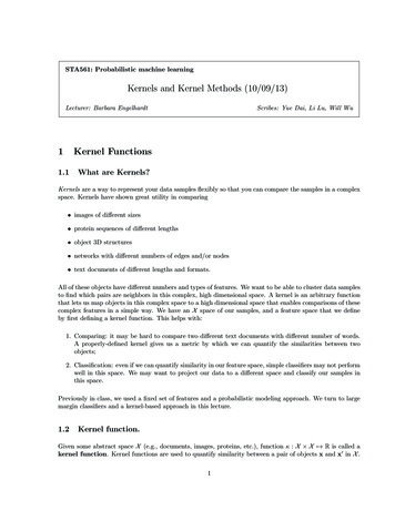
6Kernels and Kernel MethodsFigure 4: Fitting a 1D data set using D 10 uniformly spaced Gaussian prototypes, with varying lengthscale σ 2 (0.1, 0.5, 50 from top to bottom)3Applications of Kernels3.1Kernelized Machineφ(x) [κ(x, µ1 ), κ(x, µ2 ), . . . , κ(x, µD )](11)where µd X are a set of D centroids. φ(x) is called a kernelized feature vector.This vector projects a new data point x into the D-dimensional feature space by computing the similaritybetween x and each centroid µ1:D via κ(·, ·). Then we can use this kernelized feature vector for logisticregression by defining p(y x, θ) Ber(wT φ(x)).φ(x) cannot be computed using the kernel trick (see below) and must be computed explicitly, so D must bea reasonable size for computation. The kerneled feature vector quantifies the distance of a particular x toeach of the predefined centroids. This provides a simple way to define a non-linear decision boundary usinga linear classifier like logistic regression, as shown in Figure 3, using (for example) a Gaussian kernel κ withfour centroids.We can also use the kernelized feature vector inside linear regression model by defining p(y x, θ) N (β T φ(x), σ 2 ).Figure 4 shows the result of fitting a 1D data set with D 10 uniformly spaced Gaussian prototypes, withvarying length scale. σ too small (e.g. σ 0.1) overfitting. σ generalizeable (e.g. σ 0.5) right line nice generalization properties σ too large (e.g. σ 50) underfitting.