WIXLIB

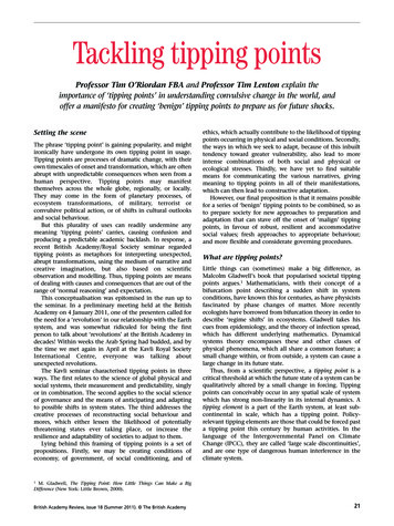
V. N. Livina et al.: Tipping point analysis91The potential can be reconstructed from time series dataof the system using the following relation to the probabilitydensity function:U (z) σ2log pd (z),2(8)which means that the empirical probability density pd (kernel distribution) has a number of modes corresponding to thenumber of wells of the potential.The structural changes of the potential are often not visible in the time series, yet they may lead to a dramatic evolution of the system. Detecting such changes gives an advantage in understanding of the dynamical system. The potentialcoloured map (Livina et al., 2010) visualizes bifurcations according to the number of detected system states. It illustratesbifurcations as the change in the colour describing the number of states along all timescales (the y axis shows the lengthof the sliding window of data for which the number of statesis assessed). If no such pattern is observed, there is no bifurcation in the time series.This stochastic approximation of the system structural dynamics has remarkable accuracy for data subsets of length asshort as 400 to 500 data points, demonstrating above 90 %rate of successful detection, as was shown in an experimentwith double-well-potential artificial data (Livina et al., 2011).For data subsets of length greater than 1000 data points it correctly detects the structure of the potential with a success rateof over 98 %.The technique of potential forecasting is based on dynamical propagation of the probability density function of the timeseries. We employ the coefficients of the Chebyshev polynomial approximation of the empirical probability distributionand extrapolate them in order to forecast the future probability distribution of the data. After reconstruction of the systemkernel distribution, a time series is generated using rejectionsampling technique, and then the obtained dataset is sortedaccording to the initial data in order to reconstruct the temporal correlations in the time series. The detailed mathematical description of the potential forecasting technique is givenin Livina et al. (2013). The technique has the advantage ofreproducing both static properties (probability density) anddynamic properties (scaling exponent, or power-law correlations) of a time series.3DataWe study the large CTBTO record (2003–2016) of the CapeLeeuwin hydrophone, series H01W1, which is a 250 Hz sampled time series of ocean sound pressure. The raw data represent 3 TB of binary waveforms, which after extraction constitute 95 billion points in the time series. We analyse 1 min averages of sound pressure level (SPL) in five frequency bands(5–115 Hz broadband as well as 10–30, 40–60, 56–70, and85–105 Hz), of about 7 million points per time series. igure 1. Initial (a) and processed (b) sound pressure level data infive frequency bands. Processing included interpolation and deseasonalization. Note that seasonal variability is less pronounced in thehigher frequencies of the initial data. At the same time, the recordsof higher frequencies have declining trend visible by eye.data have pronounced seasonality and some small gaps, andtherefore we perform interpolation and deseasonalization ofall five time series, the result of which can be seen in Fig. 1.The data samples were scaled using their calibration factors (provided by CTBTO), and an inverse filter of the recording system’s frequency response was applied to eliminate theeffect of the acquisition chain on the frequency response ofthe recordings. The fast Fourier transform (FFT) of the signalwas computed using rectangular windows of 15 000 samples(i.e. 1 min intervals at 250 Hz sampling rate) and the broadband signal was then filtered in five frequency bands (5–115,10–30, 40–60, 56–70, 85–105 Hz) via selection of the corresponding FFT bins within each frequency band. Then theresulting sound pressure level (SPL) in dB re 1 µ Pa2 for eachfrequency band was calculated (Robinson et al., 2014; ISO18405, 2017). Finally, outliers, i.e. levels more than 20 dBabove the average of the entire time series of SPL values,were removed.Because of the data gaps, we interpolate the SPL data toachieve equidistant 1 min temporal resolution. We then reNonlin. Processes Geophys., 25, 89–97, 2018

92V. N. Livina et al.: Tipping point analysisFigure 2. Trend estimation in SPL bands (deseasonalized data)using “delete-d” jackknife sampling with 1000 subsets with d 10 000 randomly deleted data points. Blue dots show the slope withcorresponding jackknife uncertainties of the least-squares linear regression, whereas red dots show the trend (the absence of it, withzero slopes of linear regression) for the shuffled data, i.e. the datawith randomly allocated values of the time series.move the seasonal periodicity by subtracting the averagedseasonal cycle over the 14 years of observation to obtain thefluctuations(9)zi Si S̄i ,where Si is the interpolated SPL data, and S̄i is the mean1 min interpolated SPL data. The resulting fluctuations areshown in the right column of Fig. 1, for the broadband andthe four selected sub-bands.4Results and discussionWe analyse the global trends of these five datasets, assumingthe simplest linear model in a least-squares regression. To estimate the uncertainty in the trends, we apply the “jackknife”technique (see Efron, 1982; Wu, 1986). We use the “deleted” variation of the method, with random subsampling andnumerical implementation reducing the number of requiredsamples, which allows to estimate variance of the trend asmmr X1Xv Tr,st Tr,skdm t 1m k 1!2,(10)where d is the number of the excluded data points in eachsample (“delete-d”) of length r n d (n is data length), Tare statistics of the trend estimator; see further details in Shaoand Tu (1995).The resulting trends show a small annual decline in SPLfor all five datasets, as shown in Fig. 2.The above trend analysis was applied to deseasonalizedfluctuations (SPL broadband). It is interesting that the average annual cycle of the initial broadband data, too, has adeclining trend, which is illustrated in Fig. 3.The origin of the seasonality in the acoustic data froma hydrophone installed at depth is a subject of discussion,because the seasonal ocean temperature fluctuations at thesurface would barely influence the sound propagation towards hydrophones. There are various possible mechanismsNonlin. Processes Geophys., 25, 89–97, 2018Figure 3. Average annual cycle of the SPL broadband, its linearregression line (red) and horizontal line (cyan) for comparison.through which seasonal variability may manifest in the hydroacoustic data. For example, seasonal variations in shipping frequency, recreational vehicle use, iceberg breakup.Seasonally, there may be a slight warming/cooling in the topfew tens of metres of water surface layer, but at the depth ofthe SOFAR (sound fixing and ranging) channel, where thehydrophone is located, temperature is stable on a seasonaltimescale. Some seasonal effects in the sound record maybe originating from iceberg formation as the edges of theAntarctic, as ice breaks up at a higher rate in the SouthernHemisphere summertime. Furthermore, seasonal variationsin whale song are plausible, as well as in fauna migrationdue to seasonal fluctuations in food supply.We next apply the pre-tipping analysis (early-warning signals) to analyse lag-1 autocorrelations and variance of thebroadband SPL record, with estimation of uncertainty. Wevary the length of the sliding windows for calculating theseindicators between one-fourth and three-fourths of the recordlength to obtain the averaged curves and standard uncertainties and display the indicator values at the end of each window, as shown in Fig. 4.The noticeable change at the end of these early-warningindicators may be related to the unusually large El Niño eventof 2015–2016. One can see that the variance decline slowsdown and autocorrelation sharply rises, which means thatthe increase in memory is not accompanied by increasingamplitude of acoustic fluctuations. Such effects may happenwhen a dynamical system experiences critical slowing downprior to a bifurcational tipping. As we hypothesize that theEl Niño signature may be related to changes in both oceanicdynamics and fauna, the increasing memory in the acousticdata may reflect, for instance, the observation that during theEl Niño the Cape Leeuwin current slows down (Feng et al.,2003). The slower ocean current introduces more inertia inthe dynamical system, and therefore higher temporal ys.net/25/89/2018/

V. N. Livina et al.: Tipping point analysis93Figure 4. Early-warning indicators of the broadband SPL dataset:lag-1 autocorrelation (upper panel) and variance (lower panel), calculated with variable window lengths, from 1/4 to 3/4 of the recordlength, and corresponding standard uncertainties, displayed at theend of each window. Both indicators demonstrate nonstationary behaviour (increasing autocorrelation and decreasing variance), whichdenotes long-term development a possible future tipping.Similar to what is seen in the CTBTO data, the effect of increasing autocorrelation and decreasing variance was earlierobserved in bifurcating artificial data changing from whitenoise to random walk, in Livina et al. (2012). The acoustics dynamics may be undergoing a similar tipping. Note thatthis analysis of early-warning signals is performed with largeenough windows (starting from a length of 3 years up to9 years), which identify large-scale variability, with possibledynamics on the scale of decades ahead.Further, we apply potential analysis to identify smallerscale variability, varying the length of the sliding windowfrom 3 days to 1 year. The resulting potential plot is shownin Fig. 5.El Niño–Southern Oscillation (ENSO) can be monitoredusing several indices, which are obtained by averaging climatic variables to make the presence of El Niño more visiblein the series. We show in Fig. 5 two of them: Southern Oscillation Index (SOI) and Oceanic Niño Index (ONI). SOI isbased on the sea level air pressure differences between Tahitiand Darwin, Australia. ONI is based on the 3-month runningmean of sea-surface temperature anomalies ERSST.v4 SST(Huang et al., 2014) in the Niño 3.4 region (NOAA SOI).Negative SOI (positive ONI) corresponds to El Niño events,characterized by warm SST in the eastern and central tropicalPacific (Trenberth and Caron, 2000).We calculate, for easier comparison of El Niño indicesand potential analysis, two binary indices derived from theONI and from the single level of the potential plot at thescale 0.5 years. The bars in the bottom panel of Fig. 5 showthe occurrence of El Niño events in the ONI (which is lessnoisy than SOI), and at the same time we plot a binary re 5. (a) Potential analysis plot of the broadband SPL data, withvarying window length (y axis) from 1 day to 1 year. The coloursdenote the number of detected potential states: green – two; cyan– three. Specks of magenta denote very short periods of a highernumber of states, which correspond to highly variable (possiblynon-potential) subsets of data of small size. (b) ENSO indices ONIand SOI, known to be anti-correlated, which indicate several ENSOevents (El Niño and La Niña). These can also be seen in the potential analysis plot. ONI positive and negative values (roughly corresponding to El Niño and La Niña) are shaded by light red and lightblue respectively, for better comparison with the indices in the lowerpanel. (c) Binary indices derived from the ONI and potential plot (atthe level 0.5 year of y-scale in the top panel) which have values 1when there is an El Niño (in the case of ONI-based binary index) oranomalous potential state (in the case of the potential binary index).dex showing periods when the system potential does not follow its “regular” three-well-potential pattern; these two indices have agreement in several periods corresponding to theknown El Niño events (2003, 2004, 2006, 2009, 2015–2016),which illustrates our hypothesis of the El Niño signature inthe acoustic data.The vertical span of the features of the potential plot (thespecks of different colours) corresponds to the timescale ofNonlin. Processes Geophys., 25, 89–97, 2018

94Figure 6. The difference between two-well-potential (first half ofthe year 2016, black curve) and three-well-potential (second half of2016, red curve) subsets of the broadband SPL record in the twoupper panels. In the lower panel, the build-up of the new potential well can be seen in the red histogram, where the main modebecomes broader and starts building two new modes around SPLvalues 3 and 0 dB re 1 Pa2 (deseasonalized SPL data).the change, i.e. the size of the time window, within whichthe change has been detected. As El Niño is a seasonal phenomenon (except the unusually long event of 2015–2016),most of such specks are located within the window of size1 year. The large event of 2015–2016, indeed, extends higherthan that. To address this timescale, we derived the binarypotential index using the detection data at fixed timescale of0.5 year, at which most El Niño events should be present inthe detection statistics.We do not claim that the potential colour plot couldbe used for early-warning signals (such as prognosis ofEl Niño), in this system or in others. Moreover, there may beother factors causing structural changes in the acoustic data,rather than El Niño or La Niña. On the other hand, detectionof such changes can indeed be useful useful for other studiesthat could investigate attribution of structural variability, andhere the technique of potential analysis might be very useful.To understand better what dynamical changes occur in theacoustic fluctuations, it is useful to plot the histograms ofthe corresponding subsets of data. Figure 6 demonstrates thedifference between the two-well-potential (first part of theyear 2016) and the three-well-potential (second part of theyear 2016) subsets, which correspond to green and cyan areasin the top panel of Fig. 5.The variability of the potential can be understood as appearance and disappearance of the SPL fluctuations, whichare present in the three-well-potential subsets and disappearin sub-periods of two-well-potential dynamics. These periods of change seem to coincide with some of the recentEl Niño events, in particular the strong oscillation in 2015–Nonlin. Processes Geophys., 25, 89–97, 2018V. N. Livina et al.: Tipping point analysis2016. Since in these short periods data become two-well potential during El Niño, one can hypothesize that the El Niñoevent reduces acoustic fluctuations events in the tails of theprobability distribution (higher and lower values) and intensifies the events in the middle range of values.It is known (Feng et al., 2003) that the Leeuwin Current isinfluenced by El Niño, which causes lower temperature andslower current. This causes a number of climatic and environmental changes (including the impact of El Niño on sea level,current transport, and migration of marine animals), and thismay affect the acoustic signal. In particular, the local sea bottom slopes near Cape Leeuwin are very steep, with large underwater peaks (see Fig. 4 in Feng et al., 2003), which maybe inducing reflection and scattering of the acoustic signal atgreater depths, where the hydrophone is located.The hydrophone, located 100 km off-coast from CapeLeeuwin at the south-western corner of Australia, has unobstructed reception of acoustic signals arriving via the SOFAR channel at angles between 110 and 355 azimuth. Thehydrophone is omnidirectional at these frequencies, but its“field of view” is blocked by the land mass of Australia. Forother azimuths, which are occluded by the Australian continental shelf, surface sounds and seismic waves can still bereflected or refracted into the SOFAR channel there wherethe ocean bottom slopes through the SOFAR channel, particularly if it does so steeply. Note that on account of thelower speed of sound in water compared to rock, refractionis towards the normal for seismic waves coupling into waterso such coupling is not efficient for a mostly horizontal seabottom: the hydrophone array will predominantly see seismic waves that impinge close to vertically from below (havea small slowness, high apparent velocity across the array)which are subsequently scattered by the wavy sea surface instead of propagating coherently onwards. Hence steep slopescouple better.The detailed analysis of directional acoustic propagation isbeyond the scope of the current paper and may be analysedlater elsewhere.Finally, we analyse the scaling properties of the deseasonalized fluctuations of the broadband SPL to identify the typeof noise present in this dynamical system. When the noise iswhite, the DFA scaling exponent has value 0.5, whereas rednoise has values of the exponent higher than 0.5 (Peng et al.,1994), with nonstationary red noise having exponent higherthan 1 (random walk has exponent 1.5). The scaling exponent is estimating by fitting the fluctuation curve F (s) s αin a log–log plot, as shown in Fig. 7. The variable “s” is thescale size of the DFA, which is the size of the varying window where the fluctuations are estimated. For more detailson the DFA method, we refer the reader to Kantelhardt et al.(2002).When we apply the scaling analysis to the deseasonalizedbroadband SPL, in both short and long temporal range it hasa high exponent (about 0.9), which means that the acoustic fluctuations are stationary red noise, and this is how theywww.nonlin-processes-geophys.net/25/89/2018/

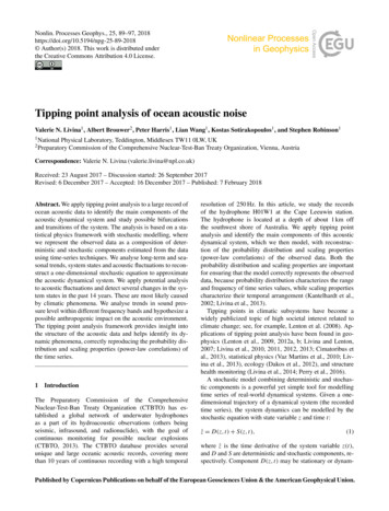
V. N. Livina et al.: Tipping point analysis95Figure 7. Detrended fluctuation analysis scaling curve of the broadband SPL, with estimated scaling exponent values. The straight linedenotes the slope with scaling exponent 1. The scaling exponentsof the curve (short term and long term) are much higher than 0.5,hence the noise is not white but red (presence of correlations); theexponent is slightly smaller than 1, which means that the fluctuations are stationary (unlike a nonstationary random walk).should be modelled to represent accurately the stochasticterm in Eq. (1).It is important to model the climatic variables with colournoise rather than with basic white noise, especially when asystem like this exhibits highly correlated long-term persistence (as estimated by DFA in Fig. 7 with α 0.96). The pattern of such fluctuations differs significantly from the patternof white noise: the persistent data (“with memory”) is likelyto have positive fluctuations tomorrow if today the fluctuations are positive. The scaling methods, such as DFA, allowone to quantify this effect, and detect the changes in the datathat are not visible in time series by a naked eye, as it is illustrated in Fig. 4. If one uses white noise for modelling suchcomplex data, the ability to analyse such data and forecast thesystem dynamics would be much reduced, with poor skill.5ModelAcoustic noise at the depth of 1 km can be influenced by multiple factors of natural and anthropogenic origin, and we investigate some of the possible components that could represent the dynamics of the acoustic system. While there may bevarious equivalent models reproducing the observed time series, we choose the simple stochastic dynamic system whichgenerates simulated time series with closely matching statistical properties.Based on the above analysis, we can formulate a stochasticmodel for the acoustic oceanic noise. We adopt an additivemodel with the following terms:ż U 0 (z, t) T (t) P (t) Figure 8. Five samples of SPL data (real, black; modelled, red).(a) Samples of data; (b) DFA scaling curves. The thin line in thepanels of the right column denotes the slope with scaling exponent 1, to which the curves are very close. The modelled data havethe same probability density and scaling properties as the real data.where U (t) is the system potential, T (t) is a long-term lineartrend, P (t) is a seasonal trend, and 8 are red-noise fluctuations. In Eq. (11), we use time as the main variable of thetime series, assuming that only the shape

The dynamics of the tipping point is forecast using extrapo-lation of the dynamically derived Chebyshev coefficients of the approximation to the probability density function of the system trajectory (Livina et al.,2013). For the purposes of potential analysis, the dynamics of the system is approximated by a potential stochastic model with