Transcription
Computational GeometryThird Edition
Mark de Berg · Otfried CheongMarc van Kreveld · Mark OvermarsComputational GeometryAlgorithms and ApplicationsThird Edition123
Prof. Dr. Mark de BergDepartment of Mathematicsand Computer ScienceTU EindhovenP.O. Box 5135600 MB EindhovenThe Netherlandsmdberg@win.tue.nlDr. Marc van KreveldDepartment of Informationand Computing SciencesUtrecht UniversityP.O. Box 80.0893508 TB UtrechtThe Netherlandsmarc@cs.uu.nlDr. Otfried Cheong, né SchwarzkopfDepartment of Computer ScienceKAISTGwahangno 335, Yuseong-guDaejeon 305-701Koreaotfried@kaist.eduProf. Dr. Mark OvermarsDepartment of Informationand Computing SciencesUtrecht UniversityP.O. Box 80.0893508 TB UtrechtThe Netherlandsmarkov@cs.uu.nlISBN 978-3-540-77973-5e-ISBN 978-3-540-77974-2DOI 10.1007/978-3-540-77974-2ACM Computing Classification (1998): F.2.2, I.3.5Library of Congress Control Number: 2008921564 2008, 2000, 1997 Springer-Verlag Berlin HeidelbergThis work is subject to copyright. All rights are reserved, whether the whole or part of the materialis concerned, specifically the rights of translation, reprinting, reuse of illustrations, recitation,broadcasting, reproduction on microfilm or in any other way, and storage in data banks. Duplicationof this publication or parts thereof is permitted only under the provisions of the German CopyrightLaw of September 9, 1965, in its current version, and permission for use must always be obtainedfrom Springer. Violations are liable for prosecution under the German Copyright Law.The use of general descriptive names, registered names, trademarks, etc. in this publication doesnot imply, even in the absence of a specific statement, that such names are exempt from the relevantprotective laws and regulations and therefore free for general use.Cover design: KünkelLopka, HeidelbergPrinted on acid-free paper987654321springer.com
PrefaceComputational geometry emerged from the field of algorithms design andanalysis in the late 1970s. It has grown into a recognized discipline with itsown journals, conferences, and a large community of active researchers. Thesuccess of the field as a research discipline can on the one hand be explainedfrom the beauty of the problems studied and the solutions obtained, and, on theother hand, by the many application domains—computer graphics, geographicinformation systems (GIS), robotics, and others—in which geometric algorithmsplay a fundamental role.For many geometric problems the early algorithmic solutions were eitherslow or difficult to understand and implement. In recent years a number of newalgorithmic techniques have been developed that improved and simplified manyof the previous approaches. In this textbook we have tried to make these modernalgorithmic solutions accessible to a large audience. The book has been writtenas a textbook for a course in computational geometry, but it can also be used forself-study.Structure of the book. Each of the sixteen chapters (except the introductorychapter) starts with a problem arising in one of the application domains. Thisproblem is then transformed into a purely geometric one, which is solvedusing techniques from computational geometry. The geometric problem and theconcepts and techniques needed to solve it are the real topic of each chapter. Thechoice of the applications was guided by the topics in computational geometrywe wanted to cover; they are not meant to provide a good coverage of theapplication domains. The purpose of the applications is to motivate the reader;the goal of the chapters is not to provide ready-to-use solutions for them. Havingsaid this, we believe that knowledge of computational geometry is importantto solve geometric problems in application areas efficiently. We hope that ourbook will not only raise the interest of people from the algorithms community,but also from people in the application areas.For most geometric problems treated we give just one solution, even whena number of different solutions exist. In general we have chosen the solutionthat is easiest to understand and implement. This is not necessarily the mostefficient solution. We also took care that the book contains a good mixture oftechniques like divide-and-conquer, plane sweep, and randomized algorithms.We decided not to treat all sorts of variations to the problems; we felt it is moreimportant to introduce all main topics in computational geometry than to givemore detailed information about a smaller number of topics.v
P REFACESeveral chapters contain one or more sections marked with a star. They contain improvements of the solution, extensions, or explain the relation betweenvarious problems. They are not essential for understanding the remainder of thebook.Every chapter concludes with a section that is entitled Notes and Comments.These sections indicate where the results described in the chapter originated,mention other solutions, generalizations, and improvements, and provide references. They can be skipped, but do contain useful material for those who wantto know more about the topic of the chapter.At the end of each chapter a number of exercises is provided. These rangefrom easy tests to check whether the reader understands the material to moreelaborate questions that extend the material covered. Difficult exercises andexercises about starred sections are indicated with a star.A course outline. Even though the chapters in this book are largely independent, they should preferably not be treated in an arbitrary order. For instance,Chapter 2 introduces plane sweep algorithms, and it is best to read this chapterbefore any of the other chapters that use this technique. Similarly, Chapter 4should be read before any other chapter that uses randomized algorithms.For a first course on computational geometry, we advise treating Chapters 1–10 in the given order. They cover the concepts and techniques that, accordingto us, should be present in any course on computational geometry. When morematerial can be covered, a selection can be made from the remaining chapters.Prerequisites. The book can be used as a textbook for a high-level undergraduate course or a low-level graduate course, depending on the rest of thecurriculum. Readers are assumed to have a basic knowledge of the design andanalysis of algorithms and data structures: they should be familiar with big-Ohnotations and simple algorithmic techniques like sorting, binary search, andbalanced search trees. No knowledge of the application domains is required, andhardly any knowledge of geometry. The analysis of the randomized algorithmsuses some very elementary probability theory.viImplementations. The algorithms in this book are presented in a pseudocode that, although rather high-level, is detailed enough to make it relativelyeasy to implement them. In particular we have tried to indicate how to handledegenerate cases, which are often a source of frustration when it comes toimplementing.We believe that it is very useful to implement one or more of the algorithms;it will give a feeling for the complexity of the algorithms in practice. Eachchapter can be seen as a programming project. Depending on the amount oftime available one can either just implement the plain geometric algorithms, orimplement the application as well.To implement a geometric algorithm a number of basic data types—points,lines, polygons, and so on—and basic routines that operate on them are needed.Implementing these basic routines in a robust manner is not easy, and takes a lot
of time. Although it is good to do this at least once, it is useful to have a softwarelibrary available that contains the basic data types and routines. Pointers to suchlibraries can be found on our Web site.P REFACEWeb site. This book is accompanied by a Web site, which contains a list oferrata collected for each edition of the book, all figures and the pseudo code forall algorithms, as well as some other resources. The address ishttp://www.cs.uu.nl/geobook/You can also use the address given on our Web site to send us errors youhave found, or any other comments you have about the book.About the third edition. This third edition contains two major additions: InChapter 7, on Voronoi diagrams, we now also discuss Voronoi diagrams of linesegments and farthest-point Voronoi diagrams. In Chapter 12, we have includedan extra section on binary space partition trees for low-density scenes, as anintroduction to realistic input models. In addition, a large number of small andsome larger errors have been corrected (see the list of errata for the secondedition on the Web site). We have also updated the notes and comments of everychapter to include references to recent results and recent literature. We havetried not to change the numbering of sections and exercises, so that it should bepossible for students in a course to still use the second edition.Acknowledgments. Writing a textbook is a long process, even with fourauthors. Many people contributed to the original first edition by providinguseful advice on what to put in the book and what not, by reading chapters andsuggesting changes, and by finding and correcting errors. Many more providedfeedback and found errors in the first two editions. We would like to thank all ofthem, in particular Pankaj Agarwal, Helmut Alt, Marshall Bern, Jit Bose, HazelEverett, Gerald Farin, Steve Fortune, Geert-Jan Giezeman, Mordecai Golin, DanHalperin, Richard Karp, Matthew Katz, Klara Kedem, Nelson Max, Joseph S. B.Mitchell, René van Oostrum, Günter Rote, Henry Shapiro, Sven Skyum, JackSnoeyink, Gert Vegter, Peter Widmayer, Chee Yap, and Günther Ziegler. Wealso would like to thank Springer-Verlag for their advice and support during thecreation of this book, its new editions, and the translations into other languages(at the time of writing, Japanese, Chinese, and Polish).Finally we would like to acknowledge the support of the Netherlands’ Organization for Scientific Research (N.W.O.) and the Korea Research Foundation (KRF).January 2008Mark de BergOtfried CheongMarc van KreveldMark Overmarsvii
Contents1 Computational Geometry1Introduction1.11.21.31.41.5An Example: Convex HullsDegeneracies and RobustnessApplication DomainsNotes and CommentsExercises2 Line Segment Intersection2810131519Thematic Map Overlay2.12.22.32.42.52.6Line Segment IntersectionThe Doubly-Connected Edge ListComputing the Overlay of Two SubdivisionsBoolean OperationsNotes and CommentsExercises3 Polygon Triangulation20293339404145Guarding an Art Gallery3.13.23.33.43.5Guarding and TriangulationsPartitioning a Polygon into Monotone PiecesTriangulating a Monotone PolygonNotes and CommentsExercises4 Linear Programming464955596063Manufacturing with Molds4.14.24.34.4The Geometry of CastingHalf-Plane IntersectionIncremental Linear ProgrammingRandomized Linear Programming64667176ix
C ONTENTS4.54.6*4.7*4.84.9Unbounded Linear ProgramsLinear Programming in Higher DimensionsSmallest Enclosing DiscsNotes and CommentsExercises5 Orthogonal Range Searching798286899195Querying a Database5.15.25.35.45.55.6*5.75.81-Dimensional Range SearchingKd-TreesRange TreesHigher-Dimensional Range TreesGeneral Sets of PointsFractional CascadingNotes and CommentsExercises6 Point Location9699105109110111115117121Knowing Where You Are6.16.26.36.4*6.56.6Point Location and Trapezoidal MapsA Randomized Incremental AlgorithmDealing with Degenerate CasesA Tail EstimateNotes and CommentsExercises7 Voronoi Diagrams122128137140143144147The Post Office Problem7.17.27.37.47.57.6Definition and Basic PropertiesComputing the Voronoi DiagramVoronoi Diagrams of Line SegmentsFarthest-Point Voronoi DiagramsNotes and CommentsExercises8 Arrangements and Duality148151160163167170173Supersampling in Ray Tracingx8.18.28.38.4Computing the DiscrepancyDualityArrangements of LinesLevels and Discrepancy175177179185
8.58.6Notes and CommentsExercises9 Delaunay Triangulations186188C ONTENTS191Height Interpolation9.19.29.39.49.5*9.69.7Triangulations of Planar Point SetsThe Delaunay TriangulationComputing the Delaunay TriangulationThe AnalysisA Framework for Randomized AlgorithmsNotes and CommentsExercises10 More Geometric Data 210.310.410.5Interval TreesPriority Search TreesSegment TreesNotes and CommentsExercises11 Convex Hulls220226231237239243Mixing Things11.1 The Complexity of Convex Hulls in 3-Space11.2 Computing Convex Hulls in 3-Space11.3* The Analysis11.4* Convex Hulls and Half-Space Intersection11.5* Voronoi Diagrams Revisited11.6 Notes and Comments11.7 Exercises12 Binary Space Partitions244246250253254256257259The Painter’s Algorithm12.1 The Definition of BSP Trees12.2 BSP Trees and the Painter’s Algorithm12.3 Constructing a BSP Tree12.4* The Size of BSP Trees in 3-Space12.5 BSP Trees for Low-Density Scenes12.6 Notes and Comments12.7 Exercises261263264268271278279xi
C ONTENTS13 Robot Motion Planning283Getting Where You Want to Be13.1 Work Space and Configuration Space13.2 A Point Robot13.3 Minkowski Sums13.4 Translational Motion Planning13.5* Motion Planning with Rotations13.6 Notes and Comments13.7 Exercises14 Quadtrees284286290297299303305307Non-Uniform Mesh Generation14.114.214.314.414.5Uniform and Non-Uniform MeshesQuadtrees for Point SetsFrom Quadtrees to MeshesNotes and CommentsExercises15 Visibility Graphs308309315318320323Finding the Shortest Route15.115.215.315.415.5Shortest Paths for a Point RobotComputing the Visibility GraphShortest Paths for a Translating Polygonal RobotNotes and CommentsExercises16 Simplex Range Searching324326330331332335Windowing Revisited16.116.216.316.416.5xiiPartition TreesMulti-Level Partition TreesCutting TreesNotes and ex377
1Computational GeometryIntroductionImagine you are walking on the campus of a university and suddenly you realizeyou have to make an urgent phone call. There are many public phones oncampus and of course you want to go to the nearest one. But which one is thenearest? It would be helpful to have a map on which you could look up thenearest public phone, wherever on campus you are. The map should show asubdivision of the campus into regions, and for each region indicate the nearestpublic phone. What would these regions look like? And how could we computethem?Even though this is not such a terribly important issue, it describes the basicsof a fundamental geometric concept, which plays a role in many applications.The subdivision of the campus is a so-called Voronoi diagram, and it will bestudied in Chapter 7 in this book. It can be used to model trading areas ofdifferent cities, to guide robots, and even to describe and simulate the growthof crystals. Computing a geometric structure like a Voronoi diagram requiresgeometric algorithms. Such algorithms form the topic of this book.A second example. Assume you located the closest public phone. Witha campus map in hand you will probably have little problem in getting to thephone along a reasonably short path, without hitting walls and other objects.But programming a robot to perform the same task is a lot more difficult. Again,the heart of the problem is geometric: given a collection of geometric obstacles,we have to find a short connection between two points, avoiding collisions withthe obstacles. Solving this so-called motion planning problem is of crucialimportance in robotics. Chapters 13 and 15 deal with geometric algorithmsrequired for motion planning.A third example. Assume you don’t have one map but two: one witha description of the various buildings, including the public phones, and oneindicating the roads on the campus. To plan a motion to the public phone wehave to overlay these maps, that is, we have to combine the information inthe two maps. Overlaying maps is one of the basic operations of geographicinformation systems. It involves locating the position of objects from one mapin the other, computing the intersection of various features, and so on. Chapter 2deals with this problem.1
Chapter 1COMPUTATIONAL GEOMETRYThese are just three examples of geometric problems requiring carefully designed geometric algorithms for their solution. In the 1970s the field of computational geometry emerged, dealing with such geometric problems. It can bedefined as the systematic study of algorithms and data structures for geometricobjects, with a focus on exact algorithms that are asymptotically fast. Manyresearchers were attracted by the challenges posed by the geometric problems.The road from problem formulation to efficient and elegant solutions has oftenbeen long, with many difficult and sub-optimal intermediate results. Today thereis a rich collection of geometric algorithms that are efficient, and relatively easyto understand and implement.This book describes the most important notions, techniques, algorithms,and data structures from computational geometry in a way that we hope will beattractive to readers who are interested in applying results from computationalgeometry. Each chapter is motivated with a real computational problem thatrequires geometric algorithms for its solution. To show the wide applicabilityof computational geometry, the problems were taken from various applicationareas: robotics, computer graphics, CAD/CAM, and geographic informationsystems.You should not expect ready-to-implement software solutions for majorproblems in the application areas. Every chapter deals with a single concept incomputational geometry; the applications only serve to introduce and motivatethe concepts. They also illustrate the process of modeling an engineeringproblem and finding an exact solution.1.1qpqpqpconvex2qAn Example: Convex HullsGood solutions to algorithmic problems of a geometric nature are mostly basedon two ingredients. One is a thorough understanding of the geometric propertiesof the problem, the other is a proper application of algorithmic techniques anddata structures. If you don’t understand the geometry of the problem, all thealgorithms of the world won’t help you to solve it efficiently. On the other hand,even if you perfectly understand the geometry of the problem, it is hard to solveit effectively if you don’t know the right algorithmic techniques. This book willgive you a thorough understanding of the most important geometric conceptsand algorithmic techniques.To illustrate the issues that arise in developing a geometric algorithm, thissection deals with one of the first problems that was studied in computationalgeometry: the computation of planar convex hulls. We’ll skip the motivationfor this problem here; if you are interested you can read the introduction toChapter 11, where we study convex hulls in 3-dimensional space.pnot convexA subset S of the plane is called convex if and only if for any pair of pointsp, q S the line segment pq is completely contained in S. The convex hullCH(S) of a set S is the smallest convex set that contains S. To be more precise,it is the intersection of all convex sets that contain S.
We will study the problem of computing the convex hull of a finite set Pof n points in the plane. We can visualize what the convex hull looks like by athought experiment. Imagine that the points are nails sticking out of the plane,take an elastic rubber band, hold it around the nails, and let it go. It will snaparound the nails, minimizing its length. The area enclosed by the rubber bandis the convex hull of P. This leads to an alternative definition of the convexhull of a finite set P of points in the plane: it is the unique convex polygonwhose vertices are points from P and that contains all points of P. Of coursewe should prove rigorously that this is well defined—that is, that the polygon isunique—and that the definition is equivalent to the one given earlier, but let’sskip that in this introductory chapter.Section 1.1AN EXAMPLE : CONVEX HULLSHow do we compute the convex hull? Before we can answer this question wemust ask another question: what does it mean to compute the convex hull?As we have seen, the convex hull of P is a convex polygon. A natural wayto represent a polygon is by listing its vertices in clockwise order, startingwith an arbitrary one. So the problem we want to solve is this: given a setP {p1 , p2 , . . . , pn } of points in the plane, compute a list that contains thosepoints from P that are the vertices of CH(P), listed in clockwise order.p9input set of points:p 1 , p 2 , p 3 , p4 , p 5 , p 6 , p 7 , p 8 , p 9output representation of the convex hull:p 4 , p 5 , p 8 , p2 , p 9p4p7p1p2p6p3p5p8The first definition of convex hulls is of little help when we want to designan algorithm to compute the convex hull. It talks about the intersection of allconvex sets containing P, of which there are infinitely many. The observationthat CH(P) is a convex polygon is more useful. Let’s see what the edges ofCH(P) are. Both endpoints p and q of such an edge are points of P, and if wedirect the line through p and q such that CH(P) lies to the right, then all thepoints of P must lie to the right of this line. The reverse is also true: if all pointsof P \ {p, q} lie to the right of the directed line through p and q, then pq is anedge of CH(P).Figure 1.1Computing a convex hullpqNow that we understand the geometry of the problem a little bit better we candevelop an algorithm. We will describe it in a style of pseudocode we will usethroughout this book.Algorithm S LOW C ONVEX H ULL(P)Input. A set P of points in the plane.Output. A list L containing the vertices of CH(P) in clockwise order.1. E 0./2. for all ordered pairs (p, q) P P with p not equal to q3.do valid true3
Chapter 1COMPUTATIONAL GEOMETRYdestination of e 1 origin of e 2e 1e 2origin of e 144.5.6.7.8.for all points r P not equal to p or qdo if r lies to the left of the directed line from p to qthen valid false. if valid then Add the directed edge pq to E.From the set E of edges construct a list L of vertices of CH(P), sorted inclockwise order.Two steps in the algorithm are perhaps not entirely clear.The first one is line 5: how do we test whether a point lies to the left or to theright of a directed line? This is one of the primitive operations required in mostgeometric algorithms. Throughout this book we assume that such operationsare available. It is clear that they can be performed in constant time so theactual implementation will not affect the asymptotic running time in order ofmagnitude. This is not to say that such primitive operations are unimportant ortrivial. They are not easy to implement correctly and their implementation willaffect the actual running time of the algorithm. Fortunately, software librariescontaining such primitive operations are nowadays available. We conclude thatwe don’t have to worry about the test in line 5; we may assume that we have afunction available performing the test for us in constant time.The other step of the algorithm that requires some explanation is the last one.In the loop of lines 2–7 we determine the set E of convex hull edges. From E wecan construct the list L as follows. The edges in E are directed, so we can speakabout the origin and the destination of an edge. Because the edges are directedsuch that the other points lie to their right, the destination of an edge comesafter its origin when the vertices are listed in clockwise order. Now removean arbitrary edge e 1 from E. Put the origin of e 1 as the first point into L, andthe destination as the second point. Find the edge e 2 in E whose origin is thedestination of e 1 , remove it from E, and append its destination to L. Next, findthe edge e 3 whose origin is the destination of e 2 , remove it from E, and appendits destination to L. We continue in this manner until there is only one edge leftin E. Then we are done; the destination of the remaining edge is necessarily theorigin of e 1 , which is already the first point in L. A simple implementation ofthis procedure takes O(n2 ) time. This can easily be improved to O(n log n), butthe time required for the rest of the algorithm dominates the total running timeanyway.Analyzing the time complexity of S LOW C ONVEX H ULL is easy. We checkn2 n pairs of points. For each pair we look at the n 2 other points to seewhether they all lie on the right side. This will take O(n3 ) time in total. Thefinal step takes O(n2 ) time, so the total running time is O(n3 ). An algorithmwith a cubic running time is too slow to be of practical use for anything but thesmallest input sets. The problem is that we did not use any clever algorithmicdesign techniques; we just translated the geometric insight into an algorithm ina brute-force manner. But before we try to do better, it is useful to make severalobservations about this algorithm.We have been a bit careless when deriving the criterion of when a pair p, qdefines an edge of CH(P). A point r does not always lie to the right or to the
left of the line through p and q, it can also happen that it lies on this line. Whatshould we do then? This is what we call a degenerate case, or a degeneracy forshort. We prefer to ignore such situations when we first think about a problem,so that we don’t get confused when we try to figure out the geometric propertiesof a problem. However, these situations do arise in practice. For instance, ifwe create the points by clicking on a screen with a mouse, all points will havesmall integer coordinates, and it is quite likely that we will create three pointson a line.To make the algorithm correct in the presence of degeneracies we must reformulate the criterion above as follows: a directed edge pq is an edge ofCH(P) if and only if all other points r P lie either strictly to the right of thedirected line through p and q, or they lie on the open line segment pq. (Weassume that there are no coinciding points in P.) So we have to replace line 5 ofthe algorithm by this more complicated test.We have been ignoring another important issue that can influence the correctnessof the result of our algorithm. We implicitly assumed that we can somehowtest exactly whether a point lies to the right or to the left of a given line. Thisis not necessarily true: if the points are given in floating point coordinates andthe computations are done using floating point arithmetic, then there will berounding errors that may distort the outcome of tests.Imagine that there are three points p, q, and r, that are nearly collinear, andthat all other points lie far to the right of them. Our algorithm tests the pairs(p, q), (r, q), and (p, r). Since these points are nearly collinear, it is possible thatthe rounding errors lead us to decide that r lies to the right of the line from p toq, that p lies to the right of the line from r to q, and that q lies to the right of theline from p to r. Of course this is geometrically impossible—but the floatingpoint arithmetic doesn’t know that! In this case the algorithm will accept allthree edges. Even worse, all three tests could give the opposite answer, in whichcase the algorithm rejects all three edges, leading to a gap in the boundary ofthe convex hull. And this leads to a serious problem when we try to constructthe sorted list of convex hull vertices in the last step of our algorithm. This stepassumes that there is exactly one edge starting in every convex hull vertex, andexactly one edge ending there. Due to the rounding errors there can suddenly betwo, or no, edges starting in vertex p. This can cause the program implementingour simple algorithm to crash, since the last step has not been designed to dealwith such inconsistent data.Although we have proven the algorithm to be correct and to handle allspecial cases, it is not robust: small errors in the computations can make itfail in completely unexpected ways. The problem is that we have proven thecorrectness assuming that we can compute exactly with real numbers.We have designed our first geometric algorithm. It computes the convex hullof a set of points in the plane. However, it is quite slow—its running time isO(n3 )—, it deals with degenerate cases in an awkward way, and it is not robust.We should try to do better.Section 1.1AN EXAMPLE : CONVEX HULLSqrpqrp5
Chapter 1COMPUTATIONAL GEOMETRYupper hullpnp1lower hullpipoints deletedTo this end we apply a standard algorithmic design technique: we willdevelop an incremental algorithm. This means that we will add the points in Pone by one, updating our solution after each addition. We give this incrementalapproach a geometric flavor by adding the points from left to right. So we firstsort the points by x-coordinate, obtaining a sorted sequence p1 , . . . , pn , and thenwe add them in that order. Because we are working from left to right, it wouldbe convenient if the convex hull vertices were also ordered from left to rightas they occur along the boundary. But this is not the case. Therefore we firstcompute only those convex hull vertices that lie on the upper hull, which is thepart of the convex hull running from the leftmost point p1 to the rightmost pointpn when the vertices are listed in clockwise order. In other words, the upperhull contains the convex hull edges bounding the convex hull from above. In asecond scan, which is performed from right to left, we compute the remainingpart of the convex hull, the lower hull.The basic step in the incremental algorithm is the update of the upper hullafter adding a point pi . In other words, given the upper hull of the pointsp1 , . . . , pi 1 , we have to compute the upper hull of p1 , . . . , pi . This can be doneas follows. When we walk around the boundary of a polygon in clockwise order,we make a turn at every vertex. For an arbitrary polygon this can be both aright turn and a left turn, but for a convex polygon every turn must be a rightturn. This suggests handling the addition of pi in the following way. Let Lupperbe a list that stores the upper vertices in left-to-right order. We first append pito Lupper . This is correct
algorithmic solutions accessible to a large audience. The book has been written as a textbook for a course in computational geometry, but it can also be used for self-study. Structure of the book. Each of the sixteen chapters (except the introductory chapter) starts with a problem arising in one of the application domains. This