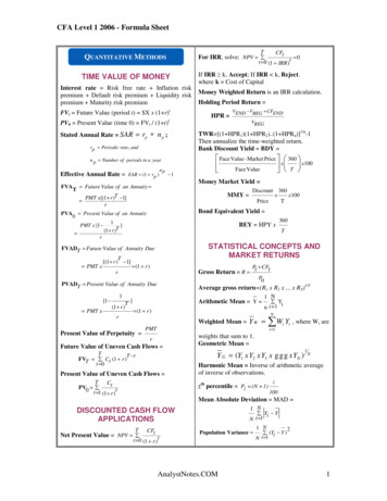
Transcription
CFA Level 1 2006 - Formula SheetQUANTITATIVE METHODSFor IRR, solve: NPV TIME VALUE OF MONEYInterest rate Risk free rate Inflation riskpremium Default risk premium Liquidity riskpremium Maturity risk premiumFVt Future Value (period t) X x (1 r)tPV0 Present Value (time 0) FVt / (1 r)trp Periodic rate, andEffective Annual Rate EAR (1 rp )FVAPVA 1Holding Period Return V V CFENDHPR END BEGVBEG r360Tx100Money Market Yield Discount 360xx100PriceTBond Equivalent Yield Present Value of an AnnuityPMT x [1 xFace ValueMMY PMT x [(1 r )T 1] r0 0Money Weighted Return is an IRR calculation.Face Value- Market Price Future Value of an Annuity Tt 0 (1 IRR )tIf IRR k, Accept; If IRR k, Reject.where k Cost of Capitaln p Number of periods in a yearnpCFtTWR [(1 HPR1)(1 HPR2).(1 HPRn)]1/n-1Then annualize the time-weighted return.Bank Discount Yield BDY rp n p ;Stated Annual Rate SART1](1 r )T360BEY HPY xTSTATISTICAL CONCEPTS ANDMARKET RETURNSFVADT Future Value of Annuity DueT[(1 r ) 1] PMT x (1 r )rP CF1Gross Return R 1PVADT Present Value of Annuity DueAverage gross return (R1 x R2 x . x RT)1/T[1 PMT x1(1 r )P0Arithmetic Mean Y T]r (1 r )Present Value of Perpetuity Weighted Mean PMTrTT tFVT Ct (1 r )t 0Present Value of Uneven Cash Flows Ct(1 r )YW NWi Yi , where Wi areweights that sum to 1.Geometric Mean Y G (Y1 xY2 xY3 x g g g xYN )1NHarmonic Mean Inverse of arithmetic averageof inverse of observations.zth percentile Pz (N 1)tz100Mean Absolute Deviation MAD DISCOUNTED CASH FLOWAPPLICATIONSNet Present Value NPV Yin i 1i 1Future Value of Uneven Cash Flows TPV0 t 11 NTCFtt 0 (1 r )t1 NYi YN i 11 N2Population Variance (Yi Y )N i 1AnalystNotes.COM1
CFA Level 1 2006 - Formula SheetSample Variance n1n 1 i 1(Yi Y )22Variance σ Covariance Standard Deviation (Variance)Target semi-variance T′( X n X TGT )n 1; such that X n X TGT1Combinatorial Formula nCr 3 ; Kurtosis of normalPermutation Formula PROBABILITY CONCEPTSPositive skewness: Mode Median MeanNegative skewness: Mode Median Mean(Positive skewness is preferred)Joint probability p(E1E2) p(E1 E2) p(E2)Addition rule of probabilities p(E1 or E2) p(E1) p(E2) – p(E1E2)Total Probability Rule p(C) p(C1 E1) p(E1) p(C2 E2) p(E2) . p(Cn En) p(En)p ( E2 E1 )Bayes Formula p(E1 E2) nExpected Value E( Y%) ][2] E Yi E (Y%)Expected Value (Total Probability Rule) E (Y%) E (Y I ) p(I ) ggg E(Y I ) p(I )KK11Variance (using conditional expectations) n2[ E ( R I i ) E ( R )]i 1n!x (p)r x (1-p)n-rr ! x (n r ) !E(Success) 2 np(1-p)f ( y) nE (Y%) p(Y I ) Y ggg p(Yn I ) Yn p(Y I ) Yi11i 1 i2(n r ) !Binomial Probability p (r successes) np1Conditional Expectation σn!Continuous Uniform Distribution: pdf p ( E2 )Variance (based on probability distribution)p Y E (Y%)i 1 i ir ! x (n r ) !Application Rule: If number of outcomes is infinite, cannot useany counting method. If n objects: n slots, all objects assigned toone slot, use factorial formula. If assigned to three or moregroups, use multinomial formula. If r objects selected withoutorder, use combinatorial formula. If r objects selected withregard to order, use permutation formula. Otherwise investigateuse of multiplication rule, or actual count.p Ys 1 i i2n!PROBABILITY DISTRIBUTIONSMultiplication rule for independence p(E1E2) p(E1 E2) p(E2) p(E1) p(E2)[ws E ( Rs )n1 ! x n2 ! x n3 ! x n4 ! x . . . x nk !distribution 3. σ s 1sY s Zn!σp4nnCovY ZMultinomial Formula R p RFSample Excess Kurtosis 2 YZMultiplication Rule of Counting n1 x n2 x n3 x n4 x n5 x . . . x nkk(Y Y )1 i 1 i4Ns][Zi E ( Z%)]σ p 2 wA 2 σ A 2 wB 2 σ B 2 2wA wB Cov ABdeviations around the mean 1 2N[p Y E (Y%)i 1 i iPortfolio Variance Chebyshev’s inequality: Proportion ofobservations in a range k (k 1) standard2]Portfolio Exp. Ret. E ( R p ) for semi-variance, replace XTGT YSharpe measure [p Y E (Y%)i 1 i iCorrelation coefficient 2T′ 1nnyU y L0for y L y yUotherwiseProperties of Normal Distribution:1. Completely described by mean and variance( , 2)2. It is symmetric with skewness measure of 0,i.e., mean mode median3. Kurtosis 3. Forms benchmark.4. Linear combinations of normal randomvariables are normally distributed.p ( Ii )AnalystNotes.COM2
CFA Level 1 2006 - Formula SheetConfidence Interval for Sample Mean:[ Y - z s/ n, Y z s/ n ]Test of Equality of Means:1. Unknown population variance assumed equal222 ( n 1) s1 ( n2 1) s2s 1( n1 n2 2)Standard Normal Variate:z Safety First Ratio y Ystn n 2 1 2E ( R p ) RTσpLognormal Distribution:ln( Y%) N ( µ , σ )2. Unknown variances assumed unequal2Continuously compounded rate ert – 1SAMPLING & ESTIMATIONCentral Limit Theorem: Irrespective of theunderlying distribution, sample means ( Y ) basedon sample size (n), have the same mean ( ) as theunderlying population, and variance that equals2/n, where 2 is the variance of the underlyingpopulation. The sample means are approximatelynormally distributed large sample sizes ( 30).Standard Error of Sample Mean: / n (population variance known)sYY s/ n (population variance unknown)(Y 1 Y 2 ) ( µ1 µ 2 )122 2s1s2 n1n222 2s1s2 n1n2modified df 2222s1s2n1n2 n1n2td f Matched Pair Test:ndi Yai Ybi ; d di 1 iEstimator Properties: Unbiasedness, Efficiency &Consistency.Student’s t-distribution: is symmetric; fatter tails;and, is characterized by degrees of freedom.sd2 n1( n 1) i 1Confidence Interval for Mean:X t/2, dfTest typeTwo-tailedOne-tailedTest Statistic (test of mean, normal distbn.)X µσ/ nType I Error: Null is Rejected when TrueType II Error: Null is Accepted when FalseY µ0sn; tn-1 ;s2d2s dnd 0sdTest of Variance Against Point Value:2 2sFn 1, n 1 L 2LSsS; (n-1) d.f.; d.f. (nL-1) & (nS-1)CORRELATION & REGRESSIONTest of Correlation (r) Against Zero:t Y µ0, (n-1) d.f.s n(n-1)s 220Test of Equality of Variances:Power of Test 1 – Type II ErrorTest of Mean:z 2nHYPOTHESIS TESTINGz ( di d )t n 1 (s/ n)Null HypothesisEqualityInequality(Y 1 Y 2 ) ( µ1 µ 2 )1211s n1 n2r n 21 r2; (n-2) d.f.Linear Regression:AnalystNotes.COMYi c 0 b 1 Xi i3
CFA Level 1 2006 - Formula SheetAssumptions: Linearity, non-randomness, zeroerror mean, homoskedasticity, uncorrelatederrors, normal errors.Potential Problems: Heteroskedasticity,Multicollinearity, Autocorrelation.Standard Error of Estimate:SEE 1n( n 2) i 1(εˆi2 )1/ 2Test of Significance of Co-efficient:t bˆ1 b10sˆ; (n-k 1) d.f.b1Analysis of Variance:TSS RSS SSEMSE SSE (n-k 1)MSR RSS kR-sq RSS TSSr R-sqF (RSS k) / [SSE (n-k 1)]; k & (n-k 1)d.f. {Test of joint significance of coefficients,i.e., regression.}SEE MSEGDP AND NATIONAL INCOMEGDP (Expenditure Approach):GDP C I G NXGDP (Resource Cost–Income Approach):GDP R T D NFGNP GDP - NFReal GDPYear T GDP DeflatorBase YearGDP DeflatorTPrice Indext - Price Indext-1Price Indext-1Natural Rate of Unemployment 1 – Fullemployment rateUnemployment: Frictional, Structural & CyclicalFiscal Policy: (1) During a recession moves the ADcurve to the right at full employment level outputbut at higher prices. (2) During boom times, AD ismoved left for full employment output at lowerprices.Crowding Out Model: Fiscal deficits whenfinanced by borrowing, raise interest rates.Neo-classical Model: When fiscal deficit is high tostimulate economy, people cut back spending inexpecting higher future taxes.Supplyside Model: Lowering tax rates increasesproductive resources and better tax collection,shifting LRAS to the right.MONETARY POLICYM1: Currency, checkable deposits and travelers’checks.M2: M1 savings deposits, money market depositsand small deposits under 100,000ECONOMICSNominal GDPT xInflation rate National Income GNP – Depreciation –Indirect taxes Personal income National income – Corporateprofits & social insurance taxes Socialsecurity, net interest and dividends received Disposable income Personal income – PersonaltaxesLong Run Aggregate Supply: Constant in shortrun. Changes when economic resources orproductivity change.Real GDP Planned consumption Plannedinvestment Planned government expenditures Planned net exportsPotential deposit expansion multiplier 1/RRRFed Policy Tools: Discount Rate; Reserve Ratio;Open Market Operation (most popular); Fed FundsRate (tracking only)Effect of Monetary Policy: Indirect throughinterest rates. Expansionary money supply in arecession lowers real interest rates spurringinvestment and consumption demand for durables,moving AD curve to the right.Money Supply Change Anticipated: If its effect isperceived to be inflationary – higher priceequilibrium results at same output.Equation of Exchange: Quantity theory of money.PxQ MxVGrowth rate of real output Rate of inflation Growth rate of money supply Growth rate ofvelocitySTABILIZATION & OUTPUTPolicy Time Lags: Recognition, Administrative,Impact.AnalystNotes.COM4
CFA Level 1 2006 - Formula SheetAdaptive expectations: Adjustment process is slowand errors are systematic.E(Xt) Xt-1 (1- ) Xt-2Rational expectations: Assumes market considersall available information like policy makersreaching the same conclusion.Activist Policy: Fiscal policy & monetary policychanges to smoothen business cycle.Non-activist Policy: Stable inflation rate, stable taxrates and stable government expenditures,irrespective of the short-run state of the economy.Government’s budget balanced over a businesscycle. Steady monetary growth to accommodategrowth in real output.SUPPLY & DEMANDConsumer Surplus: Area under the demand curvebut above the equilibrium price.Elasticity of Demand % Change in Quantity %Change in Price (midpoints)Producer Surplus: Area above the supply curvebut below the equilibrium price.Total surplus Consumer surplus ProducersurplusElasticity of Supply % Change in Quantity %Change in Price (midpoints)Shifts Along Supply and Demand Curve: Theseare caused by changes in price.Shifts in Demand Curve: Caused by factors otherthan price: consumer income, number of consumers,price of related good, changes in expectations,demographics, consumer tastes and preferences.Shifts in Supply Curve: Caused by factors otherthan price: price of resources, technology, naturaland political disruptions, tax changes, number offirms in the market.Long Run Supply Curve: Is more elastic than theshort run supply curve.Shortages and Prices: In the short run priceincreases but in the long run both the demand curveand supply become more elastic and price fallssomewhat.Prices as Invisible Hand: Communicatesinformation; Coordinates actions; Motivates marketparticipants.Price Ceilings & Floors: Ceilings create excessdemand and floors create excess supply and relianceupon non-price factors.Tax incidence: Greater proportion of actualincidence of tax is borne by the party with the moreinelastic curve: demand or supply.Choice Among Several Goods: Consumer equate:MU kMU1 MU 2 MU 3 . P1P2P3PkDeterminants of Elasticity of Demand:Availability of substitutes; Impact of time; Share ofbudget spent on a product; Consumer’s opportunitycost of time.Change in Total Consumer expenditure: (1 eP )Assumptions Behind Indifference Curves: (1)Prefer more over less, (2) Goods can be substituted,and (3) Marginal utility declines with consumption.No two indifference curves for an individual canintersect.Substitution Effect: Price increase will lead tolower consumption of the good and switching byconsumers to its substitutes.Income Effect: Change in price of a good in has thesame affect as a change in her income. Priceincrease will lead to a cutback in the consumptionof the good.COSTS AND SUPPLYEconomic Profit: It takes into account implicit andexplicit costs.Accounting Profit: Only takes into account explicitcosts.Marginal Product and Cost: Marginal productfirst increases with volume and then decreases.Marginal cost first decreases and then increases.LRATC: This is the envelope of the all possibleminimum cost points of short run average total cost.Economies of Scale: As volume increases, averagetotal cost declines.Cost Curves Shift: Due to – Resource prices,Taxes, technology, Regulation.PRICE TAKERSDemand Curve: Industry demand curve isdownward sloping and firm’s demand curve ishorizontal. Many firms, none can influence price.Equilibrium Condition: pM MR MCIf pM AVC, a firm would shut down temporarily.Long Run Equilibrium: All firms make zeroeconomic profits, andAnalystNotes.COMpM MR MC ATC5
CFA Level 1 2006 - Formula SheetPRICE SEARCHERS – LOWBARRIERSProfit Maximizing Condition: Firms face adownward sloping demand curve and maximizeprofit by settingMR MCAlso, Marginal Revenue (MR ) PriceContestable Market Implications: Due to threat ofentry, firms make zero economic profit, and price ATC.Price Discrimination: Firms charge different pricesin markets with different demand elasticities toincrease revenue and profits.PRICE SEARCHERS – HIGHBARRIERSBarriers to Entry: (1) Economies of scale, (2)Government licensing, (3) Patent rights, (4) Controlof a key resource by a firm.Monopoly: Only one firm.Oligopoly: More than one, usually less than five,firms.Profit Maximizing Condition: MR MCunder both – oligopoly and monopoly.Collusion Under Oligopoly: Price and profits arehigher. Quantity is lower. Firm has incentive tocheat by increasing output. LRATC is flat andserves as MC curve.Obstacles to Collusion: (1) Effectiveness decreasesas firms increase, (2) Monitoring and detectiondifficulty, (3) Threat of entry if low barriers, (4)Unstable demand, and (5) Antitrust and legalprosecution.Regulatory Problems in Controlling a Monopoly:(1) Imperfect information, (2) Shifting of costs, (3)Influence of special interests, and (4) Delayedresponse.Natural Monopoly: It results when there
CFA Level 1 2006 - Formula Sheet AnalystNotes.COM 1 TIME VALUE OF MONEY Interest rate Risk free rate Inflation risk premium Default risk premium Liquidity risk premium Maturity risk premium FV t Future Value -(period t) X x (1 r)t PV 0 Present Value (time 0) FV t / (1 r)t Stated Annual Rate SAR r p * n p; rp Periodic rate, and
