WIXLIB

4Authors Suppressed Due to Excessive Lengthfirst time explore a usable form of IOC-NNs, and shows that they can be trainedwith NN like capacity.– Through a set of intuitive experiments, we detail its internal functioning, especiallyin terms of its self regularization properties and decision boundaries. We show thathow sufficiently complex decision boundaries can be learned using an argmax overa set of convex functions (where each class is represented by a single convex function). We further propose a framework to learn the ensemble of IOC-NNs.– With a comprehensive set of quantitative and qualitative experiments, we demonstrate IOC-NN’s outstanding generalization abilities. IOC-MLPs achieve near zerogeneralization error in all the studied datasets and a negative generalization error(test accuracy is higher than train accuracy) in a couple of them, even at convergence. Such never seen behaviour opens up a promising avenue for more futureexplorations.– We explore the robustness of IOC-NNs to label noise and find that it strongly resistsfitting the random labels. Even while training, IOC-NNs show no signs of fitting onnoisy data and efficiently learns patterns from non noisy data. Our findings ignitesexplorations towards tighter generalization bounds for neural networks.2Related WorkSimple Convex models: Our work relates to parameter estimation on models that areguaranteed to be convex by its construction. For regression problems, Magnani andBoyd [20] study the problem of fitting a convex piecewise linear function to a givenset of data points. For classification problems, this traditionally translates to polyhedral classifiers. A polyhedral classifier can be described as an intersection of a finitenumber of hyperplanes. There have been several attempts to address the problem oflearning polyhedral classifiers [21, 15]. However, these algorithms require the numberof hyperplanes as an input, which is a major constraint. Furthermore, these classifiers donot give completely smooth boundaries (at the intersection of hyperplanes). As anothermajor limitation, these classifiers cannot model the boundaries in which each class isdistributed over the union of non-intersecting convex regions (e.g., XOR problem). Theproposed IOC-NN (even with a single hidden layer) supersedes this direction of work.Convex Neural Networks: Amos et al. [1] mentions the possibility of fully convex networks, however, does not present any experiments with it. The focus of their work is toachieve structured predictions using partially convex network (using convexity w.r.t tosome of the inputs). They propose a specific architecture called FICNN which is fullyconvex and has fully connected layers with skip connections. The skip connections area must because their architecture cannot even achieve identity mapping without them.In contrast, our work can take any given architecture and derive its convex counterpart (we use the IOC suffix to suggest model agnostic nature of our work). The workby Kent et al. [16] analyze the links between polynomial functions and input convexneural networks to understand the trade-offs between model expressiveness and easeof optimization. Chen et al. [7, 8] explore the use of input convex neural network in avariety of control applications like voltage regulation. The literature on input convex

The Curious Case of Convex Neural Networks5neural networks has been limited to niche tailored scenarios. Two key highlights ofour work are: (a) to use activations that allow the flow of negative values (like ELU,leaky ReLU, etc.), which enables a richer representation (retaining fundamental properties like identity mapping which are not achievable using ReLU) and (b) to bring amore in-depth perspective on the functioning of convex networks and the resulting decision boundaries. Consequently, we present IOC-NNs as a preferred option over thebase architectures, especially in terms of generalization abilities, using experiments onmainstream image classification benchmarks.Generalization in Deep Neural Nets: Conventional machine learning wisdom says thatoverparameterization leads to poor generalization performance owing to overfitting.Counter-intuitively, empirical evidence shows that neural networks give better generalization with an increased number of parameters even without any explicit regularization [26]. Explaining how neural networks generalize despite being overparameterizedis an important question in deep learning [26, 23].Neyshabur et al. [24] study different complexity measures and capacity boundsbased on the number of parameters, VC dimension, Rademacher complexity etc., andconclude that these bounds fail to explain the generalization behavior of neural networks on overparameterization. Neyshabur et al. [25] suggest that restricting the hypothesis class gives a generalization bound that decreases with an increase in the number of parameters. Their experiments show that restricting the spectral norm of thehidden layer leads to tighter generalization bounds.The above discussion implies that a hypothetical neural network that can fit anyhypothesis will have a worse generalization than the practical neural networks whichspan a restricted hypothesis class. Inspired by this idea, we propose a principled wayof restricting the hypothesis class of neural networks (by convexity constraints) thatimproves their generalization ability in practice. In the previous efforts to train fullyinput output convex networks, they were shown to have a limited capacity compared toits neural network counterpart [1, 3], making their generalization capabilities ineffectivein practice. To our knowledge, we for the first time present a method to formulate andefficiently train IOC-NNs opening an avenue to explore their generalization ability.3Input Output Convex NetworksWe first consider the case of an MLP with k hidden layers. The output of ith neuron(l)(l)in the lth hidden layer will be denoted as hi . For an input x (x1 , . . . , xd ), hi isdefined as:X (l)(l)(l)hi φ(wij hl 1 bi ),(1)jj(0)(k 1)where, hj xj (j 1 . . . d) and hj yj (j th output). The first hidden layer represents an affine mapping of input and preserves the convexity (i.e. each neuron in h(1)is convex function of input). The subsequent layers are a weighted sum of neurons fromthe previous layer followed by an activation function. The final output y is convex with(2:k 1)respect to the input x by ensuring two conditions: (a) wij 0 and (b) φ is convex

6Authors Suppressed Due to Excessive Lengthand a non-decreasing function. The proof follows from the operator properties [5] thatthe non-negative sum of convex functions is convex and the composition f (g(x)) isconvex if g is convex and f is convex and non-decreasing.A similar intuition follows for convolutional architectures as well, where each neuron in the next layer is a weighted sum of the previous layer. Convexity can be assuredby restricting filter weights to be non-negative and using a convex and non-decreasingactivation function. Filter weights in the first convolutional layer can take negative values, as they only represent an affine mapping of the input. The maxpool operation alsopreserves convexity since point-wise maximum of convex functions is convex [5]. Also,the skip connection does not violate Input Output Convexity, since the input to eachlayer is still a non-negative weighted sum of convex functions.We use an ELU activation to allow negative values; this is a minor but a key changefrom the previous efforts that rely on ReLU activation. For instance, with non-negativity(2:k 1)constraints on weights (wij 0), ReLU activations restrict the allowable use ofhidden units that mirror the identity mapping. Previous works rely on passthrough/skipconnections to address [1] this concern. The use of ELU enables identity mapping andallows us to use the convex counterparts of existing networks without any architecturalchanges.3.1Convexity as Self RegularizerWe define self regularization as the property in which the network itself has somefunctional constraints. Inducing convexity can be viewed as a self regularization technique. For example, consider a quadratic classifier in R2 of the form f (x1 , x2 ) w1 x21 w2 x22 w3 x1 x2 w4 x1 w5 x2 w0 . If we want the function f to be convex,then it is required that the network imposes following constraints on the parameters, w1 0, w2 0, 2 w1 w2 w3 2 w1 w2 , which essentially means that we arerestricting the hypothesis space.Similar inferences can be drawn by taking the example of polyhedral classifiers.Polyhedral classifiers are a special class of Mixture of Experts (MoE) network [13,27]. VC-dimension of a polyhedral classifier in d-dimension formed by the intersectionof m hyperplanes is upper bounded by 2(d 1)m log(3m) [30]. On the other hand,VC-dimension of a standard mixture of m binary experts in d-dimension is O(m4 d2 )[14]. Thus, by imposing convexity, the VC-dimension becomes linear with the datadimension d and m log(m) with the number of experts. This is a huge reduction in theoverall representation capacity compared to the standard mixture of binary experts.Furthermore, adding non-negativity constraints alone can lead to regularization. Forexample, the VC dimension of a sign constrained linear classifier in Rd reduces fromd 1 to d [6, 19]. The proposed IOC-NN uses a combination of sign constraints andrestrictions on the family of activation functions for inducing convexity. The representation capacity of the resulting network reduces, and therefore, regularization comes intoeffect. This effectively helps in improving generalization and controlling overfitting, asclearly observed in our empirical studies (Section 4.1).

The Curious Case of Convex Neural Networks(a)(b)(c)7(d)Fig. 2. Decision boundaries of different networks trained for two class classification. (a) Originaldata: one class shown by blue and the other orange. (b) Decision boundary learnt using MLP.(c) Decision boundary learnt using IOC-MLP with single node in the output layer. (d) Decisionboundary learnt using IOC-MLP with two nodes in the output layer (ground truth as one hotvectors).f(x)g(x)C2C1C2C1C2C1C2(a)(b)Fig. 3. (a) Using two simple 1-D functions we illustrate that argmax of two convex functionscan result into non-convex decision boundaries. (b) Two convex functions whose argmax resultsinto the decision boundaries shown in Figure 2(d). The same plot is shown from two differentviewpoints.3.2IOC-NN Decision BoundariesConsider a scenario of binary classification in 2D space as presented in Figure 2(a).We train a three-layer MLP with a single output and a sigmoid activation for the lastlayer. The network comfortably learns to separate the two classes. The learned boundaries by the MLP are shown in Figure 2(b). We then train an IOC-MLP with the samearchitecture. The learned boundary is shown in Figure 2(c). IOC-MLP learns a singleconvex function as output w.r.t the input and its contour at the value of 0.5 define thedecision boundary. The use of non-convex activation like sigmoid in the last layer doesnot distort convexity of decision boundary (Appendix A)We further explore IOC-MLP with a variant architecture where the ground truthis presented as a one-hot vector (allowing two outputs). The network learns two convex functions f and g representing each class, and their argmax defines the decisionboundary. Thus, if g(x) f (x) 0, then x is assigned to class C1 and C2 otherwise.Therefore, it can learn non-convex decision boundaries as shown in Figure 3. Pleasenote that g f is no more convex unless g 00 f 00 0. In the considered problemof binary classification in Figure 2, using one-hot output allows the network to learnnon-convex boundaries (Figure 2 (d)). The corresponding two output functions (one

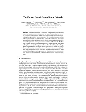
8Authors Suppressed Due to Excessive Length(a)(b)(c)Fig. 4. (a) Original Data. (b) Output of the gating network, each color represents picking a particular expert. (c) Decision boundaries of the individual IOC-MLPs. We mark the correspondencesbetween each expert and the segment for which it was selected. Notice how the V-shape is partitioned and classified using two different IOC-MLPs.for each class) are illustrated in Figure 3 (b). We can observe that both the individual functions are convex; however, their arrangement is such that the argmax leadsto a reasonably complex decision boundary.This happens due to the fact that the setsS1 {x g(x) f (x) 0} and S2 {x g(x) f (x) 0} can both be non-convex(even though functions f (.) and g(.) are convex).3.3Ensemble of IOC-NNWe further explore the ensemble of IOC-NN for multi-class classification. We exploretwo different ways to learn the ensembles:1. Mixture of IOC-NN Experts: Training a mixture of IOC-NNs and an additionalgating network [13]. The gating network can be non-convex and outputs a scalarweight for each expert. The gating network and the multiple IOC-NNs (experts) aretrained in an Expectation-Maximization (EM) framework, i.e., training the gatingnetwork and the experts iteratively.2. Boosting Gating: In this setup, each IOC-NN is trained individually. The firstmodel is trained on the whole data, and the consecutive models are trained withexaggerated data on the samples on which the previous model performs poorly. Forbootstrapping, we use a simple re-weighting mechanism as in [10]. A gating network is then trained over the ensemble of IOC-NNs. The weights of the individualnetworks are frozen while training the gating network.We detail the idea of ensembles using a representative experiment for binary classification on the data presented in Figure 4(a). We train a mixture of p IOC-MLPs witha gating network using the EM algorithm. The gating network is an MLP with a singlehidden layer, the output of which is a p dimensional vector. Each of the IOC-MLP is athree-layer MLP with a single output. We keep a single output to ensure that each IOCMLP learns a convex decision boundary. The output of the gating network is illustratedin Figure 4(b). A particular IOC-MLP was selected for each partition and led to fivepartitions. The decision boundaries of individual IOC-MLPs are shown in Figure 4(c).It is interesting to note that the MoE of binary IOC-MLPs fractures the input space intosub-spaces where a convex boundary is sufficient for classification.

The Curious Case of Convex Neural Networks49ExperimentsDataset and Architectures: To show the significance of enhanced performance of IOCMLP over traditional NN, we train them on six different datasets: MNIST, FMNIST,STL-10, SVHN, CIFAR-10, and CIFAR-100. We use an MLP with three hidden layersand 800 nodes in each layer. We use batch normalization between every layer, and it’sactivation in all hidden layers. ReLU and ELU are used as activations for NN and IOCrespectively, and softmax is used in the last layer. We use Adam optimizer with an initiallearning rate of 0.0001 and use validation accuracy for early stopping.We perform experiments that involve two additional architectures to extend thecomparative study between IOC and NN on CIFAR-10 and CIFAR-100 datasets. Weuse a fully convolutional [29], and a densely connected architecture [12]. We chooseDenseNet with growth rate k 12, for our experiments. We term the convex counterpartsas IOC-AllConv, IOC-DenseNet, respectively, and compare against their base neuralnetwork counterparts [12, 29]. In all comparative studies, we follow the same trainingand augmentation strategy to train IOC-NNs, as used by the aforementioned neuralnetworks.Training on duplicate free data: The test sets of CIFAR-10 and CIFAR-100 datasetshave 3.25% and 10% duplicate images, respectively [4]. Neural networks show higherperformance on these datasets due to the bias created by this duplicate data (neural networks have been shown to memorize the data). CIFAIR-10 and CIFAIR-100 datasetsare variants of CIFAR-10 and CIFAR-100 respectively, where all the duplicate imagesin the test data are replaced with new images. Barz et al. [4] observed that the performance of most neural architectures drops when trained and tested on bias-free CIFAIRdata. We train IOC-NN and their neural network counterparts on CIFAIR-10 data withthree different architectures: a fully connected network (MLP), a fully convolutionalnetwork (AllConv) [29] and a densely connected network (DenseNet) [12].Training IOC architectures: We tried four variations for weight constraints to enforceconvexity constraints: clipping negative weights to zero, taking absolute of weights,exponentiation of negative weights and shifting the weights after each iteration. We useexponentiation strategy in all experiments, as it gave the best results. We exponentiatethe negative weights after every update. The IOC constrained optimization algorithmdiffers only by a single step from the traditional algorithms (Appendix B).To conserve convexity in the batch-normalization layer, we also constrain the gammascaler with exponentiation. However, in practice we found that the IOC networks retainsall desirable properties without constraining the gamma scalar. We make few additionalmodifications to facilitate the training of IOC-NNs. Such changes do not affect the performance of the base neural networks. We use ELU as an activation function insteadof ReLU in IOC-NNs. We apply the whitening transformation to the input so that itis zero-centered, decorrelated, and spans over positive and negative values equally. Wealso increase the number of nodes in the first layer (the only layer where parameters cantake negative values). We use a slower schedule for learning rate decay than the basecounterparts. The IOC-NNs have a softmax layer at the last layer and are trained withcross-entropy loss (same as neural networks).

10Authors Suppressed Due to Excessive LengthTraining ensembles of binary experts: We divide CIFAR-10 dataset into 2 classes,namely: ‘Animal’ (CIFAR-10 labels: ‘Bird’, ‘Cat’, ‘Deer’, ‘Dog’, ‘Frog’ and ‘Horse’)and ‘Not Animal’. We train an ensemble of IOC-MLP, where each expert is a threelayer MLP with one output (with sigmoid activation at the output node). The gatingnetwork in the EM approach is a one layer MLP which takes an image as input andpredicts the weights by which the individual expert predictions get averaged. We reporttest results of ensembles with each additional expert. This experiment resembles thestudy shown in Figure 4.Training Boosted ensembles: The lower training accuracy of IOC-NNs makes themsuitable for boosting (while the training accuracy saturates in non-convex counterparts).For bootstrapping, we use a simple re-weighting mechanism as in [10]. We train threeexperts for each experiment. The gating network is a regular neural network, which isa shallow version of the actual experts. We train an MLP with only one hidden layer,a four-layer fully convolutional network, and a DenseNet with two dense-blocks asthe gate for the three respective architectures. We report the accuracy of the ensembletrained in this fashion as well as the accuracy if we would have used an oracle insteadof the gating network.Partially randomized labeling: Here, we investigate IOC-NN’s behavior in the presence of partial label noise. We do a comparative study between IOC and neural networks using All-Conv architecture, similar to the experiment performed by [31]. Weuse CIFAR-10 dataset and make them noisy by systematically randomizing the labelsof a selected percentage of training data. We report the performance of All-Conv, andit’s IOC counterpart on 20, 40, 60, 80 and 100 percent noise in the train data. We reporttrain and test scores at peak performance (performance if we had used early stopping)and at convergence (if loss goes below 0.001 or at 2000 epochs).4.1ResultsIOC as a preferred alternative for Multi-Layer-Perceptrons: MLP is most basic andearliest explored form of neural networks. We compare the train and test scores ofMLP and IOC-MLP in Table 1. With a sufficient number of parameters, MLP (a basicNN architecture) perfectly fits the training data. However, it fails to generalize wellon the test data owing to brute force memorization. The results in Table 1 indicatethat IOC-MLP gives a smaller generalization gap (the difference between train and testaccuracies) compared to MLP. The generalization gap even goes to negative valueson three of the datasets. MLP (being poorly optimized for parameter utilization) isone of the architectures prone to overfitting the most, and IOC constraints help retaintest performance resisting the tendency to overfit. Obtaining negative or almost zerogeneralization error even at convergence is a never seen behaviour in deep networksand the results clearly suggest the profound generalization abilities of Input OutputConvexity, especially when applied to fully connected networks.Furthermore, having the IOC constraints significantly boosts the test accuracy ondatasets where neural network gives a high generalization gap (Table 1). This trendis clearly visible in Figure 5(b). For the CIFAR-10 dataset, unconstrained MLP gives

The Curious Case of Convex Neural Networks11NNIOC-NNtraintest gen. gap traintest gen. gapMNIST99.34 99.160.1998.77 99.25-0.48FMNIST94.8 90.613.8

IOC with NN-like capacity, we, for the first time, discover the beautiful underlying properties, especially in terms of generalization abilities and robustness to label noise. We investigate IOC-NNs on six commonly used image classification benchmarks and pose them as a preferred alternative over the non-convex architectures. Our experiments