Transcription
Introduction to Plasma Physics2019 SULI One Week CourseArturo DominguezJune 12, 20191Introductory RemarksThis lecture is intended to be a brief introduction to what I consider to be theprincipal ”must know” characteristics of plasma. It is, in no way, intended tobe a comprehensive discussion of the topic. For more advanced introductionsto plasma physics, there are several good resources: eg. Introduction to PlasmaPhysics (F. Chen), Plasma Physics (R, Goldston, P. Rutherford). There arealso free online lecture notes of Intro to Plasma courses: R. Fitzpatrick at UTAustin and R. Parker at MIT (linkable on the pdf of this document).2Plasma CharacteristicsWhen gas becomes ionized it becomes a plasma. Typically, what we consider tobe a plasma is actually not fully ionized. In many cases, only a small fraction ofthe gas is ionized. These are called (not surprisingly) weakly ionized plasmas,as opposed to fully ionized plasmas (deep in the sun or inside a magneticallyconfined fusion device). The degree of ionization is determined by the SahaEquation:niT 3/2 Ui /kB T 2.4 1021e(1)nnniWhere ni and nn are the density of the ions and the neutrals in [m 3 ], T is thegas temperature in Kelvin, kB is Boltzmann’s constant and Ui is the ionizationenergy, that is, the energy required to remove the outermost electron. As acomparison, at standard temperature and pressure, nitrogen has a degree ofionization of:ni 10 122 .(2)nnAs the temperature starts rising to the order of Ui (that is, to around a fewthousands degrees K), the ionization becomes non-negligible and the gas becomes a plasma.1
3Review of basic mechanics equationsDisregarding magnetic forces, the basic equation of motion of a given particle ofmass m1 and electric charge q1 when it comes a distance r1,2 to another chargedparticle of mass m2 and charge q2 is given by the equation:#"qqGmm1212 r̂(3)m1 a ΣF F G F E 22r1,24π 0 r1,2where F G is the gravitational attraction (hence the minus sign) and F E is theelectrical force. G and 0 are the gravitational constant and the permittivity offree space respectively. Assuming particle 1 is an electron and particle 2 is aDeuterium isotope, then the ratio between the forces is:FE 1.1 1039 ,FG(4)therefore, for laboratory plasmas, gravitational forces can be disregarded andwe can focus only on electric and magnetic forces, otherwise called the LorentzForce. Note that gravity IS important for astrophysical plasmas due to the lowdegree of ionization and size of the systems.For a particle of mass m and charge q moving with a velocity v through an and B respectively, the equation ofelectric and magnetic field of magnitudes Emotion of the particle is:hi v B F m a q E(5)This is the equation we will use when analyzing the mechanics of individualparticles in the plasma.4Plasma thought experimentLet’s begin with a simple picture of a rectangular box of plasma which, asquasi-neutrality dictates, is composed of electrons and positive ions, as shownin Figure 1.4.1Plasma FrequencyNow suppose we are to move the center of mass of the electrons to the left (ornegative direction in our x̂ axis) a distance x. There is now an accumulationof electrons on the left and an accumulation of ions on the right. An electricfield is therefore created which points away from the positive slab and towardsthe negative slab. In fact, if we imagine the distance between the positive andnegative slabs to be very small compared to the area of the slabs, then theboundary conditions are too far from our points of interest and we can view2
F x eE Ex̂xFigure 1: Moving the center of mass of the electrons with respect to the ionscreates a restoring forcethis as an ideal parallel plate capacitor.The electric field inside an ideal parallel plate capacitor is simply: σ Q/A (ene A x)/A ene xE 0 0 0 0(6)pointing in the negative direction, where σ is the surface charge density (chargeper unit area) of the plate, or slab in this case, Q is the total charge of the slaband A is its area. Note that the electric field is uniform between the slabs andit does not depend on their area, only on their thickness and number density.The most common way of finding the electric field in a capacitor is done using ρ/ 0 , where, in our case, ρ ene is the volume chargeGauss’ Law: · Edensity. We won’t go into detail here, but this is a very beautiful derivationwhich uses the symmetry of the system.Now, if we have an electron in the middle of the box feeling the electric field,the force on this electron (which, as with all of the electrons in the slab, hasbeen shifted in the x̂ direction), is:22 e ne ( x) a e ne xF e me a eE 0me 0(7)Where I have incorporated the direction of the shift in to the x vector. ButEquation 7 is simply that of a harmonic oscillator with frequency:se2 neωpe (8)me 03
Figure 2: The pressure difference between two vertical positions is related tothe weight of the slab between them.Not surprisingly this is the electron plasma frequency of the system. Analogously, for an ion pof charge Ze and mass mi , the ion plasma frequency can bedefined as: ωpi (Z 2 e2 ni )/(mi 0 ). Let’s look at it in a little more detail: Ifyou look at the thought experiment, for the same displacement, the total chargein each slab will increase as you increase the electron number density ne , hencethe force is stronger and our oscillation is faster. Also, for the same field, theacceleration on electrons is greater than that of ions because the same force is excerpted on such disparate masses. This explains the inverse relation(eE)on mass.4.2Thermal VelocityNow, let’s forget about the thought experiment for a second and think aboutthe individual moving particles in our system. As energy is given to the plasma(through external voltages, neutral particle bombardment, microwave heating,etc.), the particles will start accelerating and colliding with each other. Afterenough time, the plasma reaches thermal equilibrium. While we have an intuitive idea of what thermal equilibrium means, how does it reflect in the state ofthe system?In the following section we will explore the concept of temperature and relate itto the density and distribution function of the plasma. This is will mostly followthe treatment from Feynman’s Lectures Vol.1. While the following analysis isdone on gas, it can be extended to plasmas.Assume a column of ideal gas in thermal equilibrium (Figure 2). It obeys theideal gas law:pV N kT(9)where p is the pressure, V is the volume, N is the total number of particles, Tis the temperature and k 1.38 10 23 JK 1 is the Boltzmann constant. Thisequation can be rewritten as:p NkT nkTV4(10)
where n is the number density of the gas.If the column is subject to gravity, the pressure at h1 should differ from thatat h1 h just by the pressure exerted by the weight of the slab between the2 heights:p(h1 ) p(h1 h) M g/A(11)p(h1 ) p(h1 h) ρV g/A(12)p(h1 ) p(h1 h) mnA hg/A(13) (p(h1 h) p(h1 ) ) mng h(14)mng hmg hkT(15) kT (n(h1 h) n(h1 ) ) n n(16)where M is the mass of the slab between the horizontal planes, ρ is the massdensity of the gas, V is the volume of the slab, A is the area of the planes, andm is the mass of the gas particles. Taking the limit of h 0, Equation 16leads to:mghkTmgh n(h 0) e kTln n n(h)C (17)(18)But the mgh numerator in the exponent of the RHS of Equation 18 is simplythe potential energy of the particles at that position (for example, the potentialenergy of an electron in a potential Φ: P.E. eΦ). So Equation 18 can begeneralized as: P.E.n( x) n0 e kT(19)assuming the potential energy is a function of a generalized position x. This isa powerful equation and we will come back to it in later sections.Now that we have the dependence of density on position (as a proxy of thepotential energy) in a thermalized gas, let’s explore its dependence on velocity.We can assume that the dependencies are separable. That is,n( x, v) f ( x)g( v )(20)where f and g are functions of only position and velocity respectively. Goingback to the column of thermalized gas, we will now explore a different question:What is the relationship between the number of particles that cross verticallyupwards at 2 different planes h1 and h2 as shown in Figure 3? It is clear that notall particles that cross h1 will reach h2 since some will not have enough energy.This is the reason that it’s more tenuous at higher P.E. In order to reach, theparticles will have to have a vertical velocity v greater than a minimum value usuch that: 1/2mu2 mg h. In other words:N(h2,v 0) N(h1,v u)5(21)
Figure 3: The particles crossing plane h2 upwards must have had a verticalvelocity of at least u (where mg h 1/2mu2 ) as they crossed plane h1where N(h2,v 0) is the number of particles crossing plane h2 upwards per unittime, and N(h1,v u) is the number of particles crossing plane h1 upwards perunit time with vertical velocity greater than u.We can look now at the number of particles crossing both planes with the samevelocity restriction: v 0, that is, we can compare N(h2,v 0) and N(h1,v 0) .As stated in Equation 20, the density can be separated between the positionaldependence and the velocity dependence. Since we’ve imposed the same velocityrestriction (v 0): 1/2mu2N(h2,v 0)n(h2) mgh e kT e kTN(h1,v 0)n(h1)(22)Finally, we can substitute Equaiton 21 into Equation 22 to get:N(h1,v u)N(h1,v 0) 1/2mu2N(v u) e kTN(v 0) e 1/2mu2kT N(v u) e(23) 1/2mu2kT(24)where we have used, again, the separable nature of the density. That is, thepositional dependence cancels out. At any height, the number of particles cross2ing the vertical plane upwards per unit time is proportional to exp( 1/2mu).kTEquation 24 is independent of position and should apply everywhere in space.We can now introduce the probability distribution function: f (v) such thatf (v)dv will be the probability that the particles have a velocity between v andv dv. Equation 24 sets a constraint on f (v). But the number of particlescrossing a given plane per unit time, T , with speed v u are not just:Z N(v u) 6 f (v)dv(25)u6
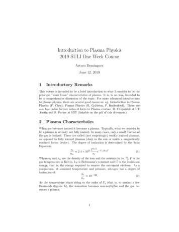
as one could intuitively think, since this would not take into account that withina unit time T , particles with velocity v will only cross the plane if they’re withina distance vT beneath the plane (slow ones have to be closer than fast ones).For a given velocity v, the number of particles a distance vT below the planewould be (vT )f (v), therefore, for all v u we have the equation:Z 1/2mu2(26)N(v u) vf (v)dv e kTuUsing the normalization:R f (v)dv 1, Equation 26 leads to:rf (v) m mv2e 2kT2πkT(27)We can extend this to 3-dimensional velocity space as: m 3/2f (vx , vy , vz ) e2πkT 2 v 2 v 2 )m(vxzy 2kT(28)We now bring back the (x, y, z) dependence: From Equation 20, we can separatethe distribution function into a positional component and a velocity-dependentcomponent:f (x, y, z, vx , vy , vz ) f x (x, y, z)f v (vx , vy , vz )(29)with a normalization:Z Z Z f (x, y, z, vx , vy , vz )dvx dvy dvz n(x, y, z) (30) Leading to the full Maxwell-Boltzmann distribution function: m 3/2ef (x, y, z, vx , vy , vz ) n(x, y, z)2πkT 2 v 2 v 2 )m(vxyz 2kT(31)What Equation 31 says is that the velocity of the particles are distributedin a Gaussian or bell curve with a width proportional to the temperature of thegas. Or, put it another way, the width of distribution in velocity space is whatgives rise to the concept of temperature of a gas.qIf we want to study the speed distribution of the particles, v v vx2 vy2 vz2 ,we find the more typical form of the the Maxwell-Boltzmann distribution function:hi m 3/22 mv(32)v 2 e 2kTf (v) 4πn02πkTan example of which is shown in Figure 4 (note that the density has been takenas homogeneous, n0 , to simplify the analysis). As is clear, the temperatureof the gas is relatedto the width of the distribution as well as to the averagepspeed vmean 3kT /m, and the most probable speed (the peak of the curve)7
Figure 4: Maxwell-Boltzmann distribution function of Argon gas at differenttemperatures. The x̂-axis is proportional to the speed of the atoms. Note thatthe area under the curve must be 1.pvpeak 2kT /m. There is, therefore, a characteristic speed of the particleswhich we call the thermal speed defined as:rkT(33)vt mNow,the electrons andpp ions will have their own thermal speeds given by: vte kTe /me and vti kTi /mi . How do these speeds typically compare?Let’s say an electron and an ion are getting energy from an electric field (whichis often the case) for a given amount of time t. The momentum gained by bothparticles is the same: me ve mi vi eEt. so ve /vi mi /me 1. Thisdisparity translates to vte and vti hence, if energy transfer between species islow, Te /Ti mi /me 1. Note that even if the particles have enough timeto reach thermal equilibrium, which is more common in magnetically confinedplasmas, Te Ti still leads to vte vti .4.3Debye LengthWe can go back to our thought experiment with the added knowledgeplasma thermal speeds. The first, and easiest way, of arriving at thelength is to do a dimensional analysis of what we’ve already acquired.found a characteristic [time] in the ωp , and we’ve found a characteristic8of theDebyeWe’vespeed,
or [length]/[time] in vt . Therefore, we can immediately deduce a characteristiclength called the Debye length:qskTvtkT 0mλD q 2 (34)ωpq2 nq nm 0More generally, the Debye length for a single species ion of charge Ze is definedas:sk 0λD (35)e2 (ne /Te Z 2 ni /Ti )which can be derived from a more detailed analysis of Poisson’s equation to beexplored later. Nonetheless, when we can take the ions as stationary (particularly in weakly ionized cold plasmas), the Debye length is effectively taken asthe electron Debye length:rkTe 0.(36)λD e2 neTo get a more intuitive picture of what the Debye length is related to, we cango back to the thought experiment where we now have a picture of an electronthat is subject to a simple harmonic oscillator system. If we were to follow themotion of the electron in this simple picture, it would follow a harmonic motionof the form:x A cos (ωpe t)(37)where I have disregarded any phase and I still haven’t determined it’s amplitude.How can we determine the amplitude A of oscillation? If we take the timederivative of Equation 37, we can find the velocity of the electron:v Aωpe sin (ωpe t)(38)But we know that the speed of the electrons is around vthe (of course, this is acharacteristic speed), so we can use that as the constraint and we haveAωpe vte A vte /ωpe λDe .(39)Where we have recovered the result found from dimensional analysis.We can derive the Debye length more rigorously by assuming a systemwherein a point charge Q is immersed in a steady state plasma (see Figure5). We can explore the electric potential Φ(r) by using Poisson’s equation: 2 Φ(r) 11ρ (ρc ρp ) 0 0(40)Where the point charge is located a the origin, hence it creates a charge density of ρc Qδ(r 0), ρp is the charge density created by the plasma, which9
Figure 5: The charge density of a system with a point charge Q immersed in aplasmawe assume is composed of electrons and a single species of ions of charge Ze:ρp ρi ρe e(Zni ne ) and Φ(r) is the electric potential, which, because ofthe symmetry of the system, we take as only a function of the radial position,r, around the point charge. Since the electrons and ions have a potential energy of eΦ and ZeΦ respectively, we can use Equation 19 assuming thermalequilibrium within each species:eΦne n0e e kTeni n0i e ZeΦkTi(41)(42)where n0e and n0i are the electron and ion densities far from the point charge(Φ 0) where quasi-neutrality prevails, so n0e Zn0i . Assuming eΦ kT : eΦne n0e 1 (43)kTe ZeΦ(44)ni n0i 1 kTi en0e ΦZ 2 enoi Φρp e n0e Zn0i (45)kTekTi e2 Φ n0eZ 2 noiρp (46)kTeTicombining Equations 40 and 46, we have: e2 n0ez 2 noiQ1Q 2 Φ(r) Φ(r) δ(0) Φ(r) δ(0)2k 0 TeTi 0λD 0(47)where we have used the definition of Debye length from Equation 35. We can10
Figure 6: The plasma shields the point charge and lowers the electric potentialclose to the chargerewrite this equation as: 1 2λD2 Φ(r) eδ(0) 0(48)before we solve this, note that if the second term in the LHS were not there, wewould recover the equation for the electric potential of a point charge: Φc (r) Q4π 0 r . The solution of Equation 48 is of the form:Φ(r) Qe (r/λD )4π 0 r(49)Figure 6 illustrates the effect the presence of the plasma has on the potentialas compared to a point charge in empty space. In the presence of a positivecharge, the electrons will quickly try to shield it, but since they are moving sofast (vte ) and in all directions, there is a region close to the charge where theelectrons will escape (due to their own inertia) and not completely shield it.This region, where the electric fields are not completely shielded, is called thesheath and its length is of the order of the Debye length.11
SystemInterstellar gasSolar WindVan Allen beltsIonosphereSolar CoronaCandle flameNeon lightsGas DischargeProcess PlasmaFusion ExperimentFusion ReactorLightningElectrons in metalne [m 3 Te [eV ]11010210 110210 112102103104310 2ωpe [s 1 ]105105106107108109109101110111011101210141016λD [m]1010110 210 310 410 410 510 410 410 410 810 12Table 1: Plasma Frequency and Debye length for various systems5Plasma frequency and Debye length for various plasma systemsIn Table 1 it’s possible to view the wide range of density and temperature whereplasma exists. The plasma frequency and Debye length has been calculated togive a sense of the characteristic parameters in the systems.The Electrons in metal case leads to an interesting discussion, outlined inFeynman’s Lectures on Physics VII 32-7 (linked in the pdf) where the reflectionand transparency of metals to electromagnetic waves can be viewed through thelens of plasma: Visible light has a frequency of 5 1014 Hz whereas xrays, forexample, have a frequency of 1016 1019 Hz.Finally, as illustrated in Figure 7 the ωpe of the ionosphere (107 Hz) leads todistinct behavior between AM and FM radio waves. It explains the reflection ofAM waves (where ω ωpe ) and the penetration of FM waves (where ω ωpe ).5.1Collisional frequencyThe final parameter to consider in an unmagnetized plasma is the frequency ofcollisions. I’ll focus on electron-electron collisional frequency (noted hereafteras νe ) but most of the dependencies and arguments are identical in ion-ion andelectron-ion collisions.The first step is to define two quantities: the time between collisions whichis the inverse of the collisional frequency, t 1/νe and the mean free path,λmf p . As we’ve seen before, the electrons are traveling at a characteristic speedof vthe , therefore, we can define:λmf p vthe t vthe /νe12(50)
Figure 7: The AM spectrum is well below the 10M Hz ωpe of the ionosphere,leading to their reflection. FM waves, at higher frequency, penetrate it.Figure 8: The volume associated with an individual electron is given by V 1/ne .13
as the distance traveled by an electron (on average) before it collides with another electron.Every electron has an associated volume in the system V 1/ne , that is, Vis the volume that is occupied by each electron. Therefore, we can define theelectron-electron cross section, σee , with the equation V σee λmf p , as shownin Figure 8. Therefore, using Equations 50 and 33:νe ne vthe σee .(51)An estimate of the cross section can be made by observing that an electronelectron collision is really a Coulomb repulsion interaction. The distance ofclosest approach, b, between colliding electrons can be taken as the radius ofthe cross section, that is:σee πb2 .(52)While the actual distance of closest approach between two colliding electronsdepends on relative velocities and angles of approach (and a rigorous derivationwould take all possible angles and velocities into account and weight them according to the distribution function), we can make a heuristic case and assumea typical configuration of an electron approaching a stationary electron head onwith a speed of vthe as in Figure 9. As shown in the figure, in the center of massframe, each electron is approaching the other with speeds vthe /2 and at closestapproach, they are separated by b. From conservation of energy, assuming thatthe electrons are very far from each other at the beginning:me (vthe /2)2me (vthe /2)2 22e2b 2π 0 me vthe e24π 0 be2.π 0 Te(53)(54)Not surprisingly, the larger the temperature, the closer the electrons can approach. Putting Equations 54 together with 52 and 51, we get the final result: p e2 2ne e4νe neTe /me 1/2 3/2Teme Te(55)since we know that many assumptions have been made, we’ve disregarded theconstants.Since the resistivity, η, is proportional to the collisional frequency, we get thevery important result:η Te 3/2(56)that is, the plasma becomes a better conductor as the temperature goes up.This dependance is of great importance in astrophysical plasmas as well as intokamak plasmas.As a point of comparison, the resistivity in a metal is well known to increasewith temperature (contrary to the case in plasmas).14
Figure 9: An electron with speed vthe colliding with a stationary one can beviewed in the center of mass frame and the distance of closest approach can bederived from conservation of energy.6Magnetized plasmasFinally, we’ll do a small introduction to what happens when we incorporateeffects of magnetic fields on the plasma. As shown in Equation 5, the force of aparticle which is moving in a magnetic field is of the form: a q ( v B) F m a q v Bm(57)Suppose a positively charged particle of mass m and charge q is moving in pointingthe plane of the paper with velocity v and there is a magnetic field Binto the paper. As shown in Figure 10, the force, hence the acceleration of theparticle is always pointing towards a center of motion and the particle draws acircular orbit in the plane. From Equation 57, the magnitude of the accelerationis a qvB/m. But we know from kinematics that if a particle is rotating arounda fixed point, the acceleration must be centripetal and the magnitude shouldbe:v2qvBvma r (58)rmqBIf the particle that is rotating is an electron (ion) with speed vte (vti ) then theradius of rotation is called the electron (ion) gyro-radius or Larmor radius andthe equations are as follows:ρe me vtemi vti, ρi eBZeB(59)Finally, we can figure out the frequency of rotation of an electron or ion that isrotating at thermal speeds: vt ωc ρ. These frequencies are very important inmagnetized plasma physics and are called electron and ion gyro-frequencies (or15
Figure 10: Trajectory of a positively charged particle moving with a velocity vwhere there is a magnetic field pointing into the page.cyclotron frequencies):ωce vtevteZeBeB me vte , ωci ρemmieeB(60)If the particles are not confined to the plane perpendicular to the magneticfields but can move in three dimensions, the particles move freely in the direction parallel to the magnetic field but are confined to move in circular orbitsperpendicular to the fields, therefore, they trace spiral orbits around the magnetic fields, as shown in Figure 11.16
electronIonFigure 11: In three dimensions, particles follow spiral trajectories around magnetic fields.17
density. We won't go into detail here, but this is a very beautiful derivation which uses the symmetry of the system. Now, if we have an electron in the middle of the box feeling the electric eld, the force on this electron (which, as with all of the electrons in the slab, has been shifted in the x direction), is: F e m e a eE e 2n e .