WIXLIB

2The Lagrangian formalism for classical mechanics: 8/31/175The homogeneity of space, told to us by invariance under the Galilei translations q j 7 q j ε, tells us thatδL L q̇ j·εi εddt L q̇ j 0.Thus, the quantityNp : L q̇ jj 1is conserved, and is constant. This is called the total momentum, so translation-invariance gives youconservation of momentum. In the same way, rotation-invariance around any center gives you conservationof angular momentum around any center.Hamiltonian dynamics The Euler-Lagrange equations express q̈ as a second-order ODE. One might wantto reformulate this into a first-order ODE; there are many ways to do this. There’s one that’s particularlyimportant. Sincepj L(q, q̇), q̇ jthen it looks like one could solve for q̇ in terms of p and q.Lemma 1.2. Let f C2 (Rn , R) be such that its Hessian D2 f is uniformly positive definite, i.e. there’s an α 0such that 2 fD2 f ( x )(h, h) h j h α k h k2 x xj i,juniformly in x Rn , then there is a unique solution toD f (x) yfor every y Rn .Proof. Let g( x, y) : f ( x ) h x, yi. Then, x g( x, y) f y, and D2 g D2 f . Hence it suffices to checkfor y 0.The positive definite assumption on D2 f means f is strictly convex, and hence has at most a singlecritical point, at which f 0. Thus it remains to check that there’s at least one solution.If you Taylor-expand, you get that1f ( x ) f (0) h D f (0), x i D2 f (sx )( x, x ) · · · ,2so for all x,f ( x ) f (0) f (0) x α 2 x .2Thus, there’s an R 0 such that if x R, then f ( x ) f (0), so f has at most one minimum in the ballBR (0), so by compactness, it has a minimum x0 , which must be the global minimum, so D f ( x0 ) 0. Definition 1.3. Suppose f is continuous on Rn . Then, its Legendre transform or Legendre-Fenchel transform isf (y) : sup (hy, x i f ( x )).x RnYou can think of this as measuring the distance from the graph of f to the line cut out by hy, x i (i.e.between the two points with minimum distance).

M393C (Topics in Mathematical Physics) Lecture Notes6Lecture 2.The Hamiltonian formalism for classical mechanics: 9/5/17Last time, we discussed Lemma 1.2, that if f : Rn R is C2 and its Hessian is uniformly positivedefinite, then there’s a unique solution to f ( x ) y for all y Rn . We then defined the Legrendre-Fencheltransform of f : f (y) geometrically means the minimal distance from f ( x ) to the hyperplane hy, x i 0. Ithas the following key properties:Theorem 2.1. Let f : Rn R be a C2 function with uniformly positive definite Hessian. Then,(1)f (y) hy, x (y)i f ( x (y)),where x (y) is the unique solution to f ( x ) y guaranteed by Lemma 1.2, and(2) f (y) is C2 and strictly convex.(3) If n 1, ( f ) ( f ) 1 .(4) For all x, y Rn ,f ( x ) f (y) hy, x i,with equality iff x x (y) is the unique solution to f ( x ) y.(5) The Legendre-Fenchel transform is involutive, i.e. ( f ) f .We’ll use this in the Hamiltonian formalism of classical mechanics. One motivation for the Hamiltonianformalism is that the Lagrangian formalism produces second-order ODEs, and it would be nice to have anapproach that gives first-order equations. There are many ways to do that, but this one has particularlynice properties.Suppose we have generalized coordinates q and p q̇L . You might ask whether we can solve forq̇i q̇i (q, p). If we assume Dv2 L(q, v) is uniformly positive definite, then p q̇ L(q, q̇) has a uniquesolution.Definition 2.2. The Hamiltonian H is the Legendre-Fenchel transform of L for q fixed, i.e.H (q, p) : sup (hp, vi L(q, v))v Rn hp, q̇(q, p)i L(q, q̇(q, p)).Theorem 2.3. Assume the matrix (2.4) 2 L q̇i q̇ j is uniformly positive definite. Then, the Euler-Lagrange equations L L 0 q̇ qare equivalent toq̇ (2.5) H, pṗ H. q(2.4) is called the mass matrix of the system, and (2.5) is called the Hamiltonian equations of motion.Proof. Since p j L q̇ j ,n q̇ j H L q̇ j q̇i p j pi pi q̇ j pij 1 q̇i .!

2The Hamiltonian formalism for classical mechanics: 9/5/17Similarly, since q j qi δij and L q̇ j7 p j , thenn q̇ j L q j L q̇ j p j qi q j qi q̇ j qij 1 L ṗi . q̇i H qi! This leads to the Hamiltonian formalism, which starts with the Hamiltonian and works towards thephysics from there. We begin on a phase space R2n with coordinates (q, p), and a Hamiltonian H : R2n R.Let 0 1nJ : 1n0denote the symplectic normal matrix.1The Hamiltonian vector field for this system is p HX H : J H . q HThen, the Hamiltonian equations of motion (2.5) may be expressed in terms of the flow for X H .This “Hamiltonian structure” on R2n is closely related to a complex structure: J 2 1 is closelyreminiscent of i2 1. Indeed, ifz : (q ip),theni ż i (q̇ i ṗ) i ( p H i q H ) ( q i p ) H.This is an example of a Wirtinger derivative:1( x i y)21 z ( x i y)2 z Example 2.6 (Harmonic oscillator). LetH (q, p) 1 2 1 2q p ,22soH (z, z) 1zz.2In this case, the Hamiltonian equations of motion arei ż 2 z H zz (0) z0 ,so we recoveras usual for a harmonic oscillator.z(t) z0 eit ,(We can also study Hamiltonian PDEs, which include several interesting systems of equations. But theygot erased before I could write them down. :( One of them includes the nonlinear Schrödinger equation: forx Rd , the system ˆ 11H[u, u] u 2 u 2p dx,22p1More generally, one can formulate this system on any symplectic manifold, in which case J is the symplectic form in Darbouxcoordinates. But we won’t worry about this right now.

M393C (Topics in Mathematical Physics) Lecture Notes8which leads to the equations of motion (the Schrödinger equation)i u̇ u u 2p 2 u.The solutions of these equations tend to be interesting: Hamiltonian flow (the flow generated by X H ) isn’t agradient flow, but rather gradient flow twisted by J. We call this flow Φt : R2n R2n , with x (t) Φt ( x0 )and x (t) Φt,s ( x (s)).Theorem 2.7. H is conserved by Φt .Proof.dH ( x (t)) x H · ẋ x H · J x H 0,dtbecause J is skew-symmetric. Definition 2.8. In this situation, the symplectic form is the skew-symmetric form ω Λ2 ((R2n ) ) defined byω ( X, Y ) : hY, JX i.The pair (R2n , ω ) is a symplectic vector space; the space of invertible matrices preserving this form iscalled the symplectic groupSp(2n, R) : { M GL2n (R) MT J M J }.Now we can prove some properties of the Hamiltonian flow.Theorem 2.9. Let Φt be the Hamiltonian flow generated by X H . Then,(1) x (t) Φt,s ( x (s)),(2) Φs,s id, and(3) DΦt,s ( x ) Sp(2n, R).Conversely, if Φt,s is the local flow generated by a vector field X such that locally (in x) (3) holds, then X is locallyHamiltonian, in that there’s a G such that X XG .Definition 2.10. A diffeomorphism φ : R2n R2n with Dφ Sp(2n, R) is called a symplectomorphism.Proof sketch of Theorem 2.9. Since t DΦt,s ( x ) DX H (Φt,s ( x )) · DΦt,s ( x ),then it suffices to check that ifΓ(t, s, x ) : DΦTt,s ( x ) JDΦt,s ( x ),thendΓ 0.dtDefinition 2.11. The Liouville measure µ L on R2n is the measure induced by ω n , i.e.ˆˆf dµ L : f ω n .R2nR2nTheorem 2.12 (Liouville). Let Φt,s be the Hamiltonian flow. Then, for every Borel set B, Φt,s ( B) B . HenceΦt,s preserves the Lesbegue measure and the Liouville measure.Proof. If ϕ : R2n R2n is a diffeomorphism, thenˆˆf ( x ) dx Bϕ 1 ( B )and det DΦt 1.( f ϕ) det Dϕ( x ) dx, The next theorem is a conservation property.Theorem 2.13. Let Φt,s be the flow generated by an arbitrary vector field X, D R2n be a bounded region, andDt,s : Φt,s ( D ). Then, for every f C1 (Rn ),ˆˆdf dx ( t f div( f X )) dx.dt Dt,sDt,s

2The Hamiltonian formalism for classical mechanics: 9/5/179Proof. By the group property (Φt,s Φt,s1 Φs1 ,s ) it suffices to prove it for s 0 and at t 0. In this caseˆˆddf dx ( f Φt ) det DΦt dxdt t 0 Dtdt t 0 DSince DΦt 1 tDX O(t2 ), then det( DΦt ) 1 t tr( DX ) O(t2 ) and henceˆ (( f f · X ) f div X ) dxˆD ( t f div f X ) dx. DCorollary 2.14. Any function f (t, x ) for which the matter contentˆMC( f )(t) : f ( x, t) dxΦt,s ( D )remains constant (equivalently,ddt MC( f )( t ) 0), must satisfy the continuity equation t f div( f X ) 0.(2.15)In physically interesting cases, the matter content actually represents how much mass is in the system.In the Hamiltonian case, div X H 0, so t f f · X H 0is equivalent to t f f · J H 0.We can rewrite this in terms of the Poisson bracket{ f , H } : h f , J H i,producing the equation t f { f , H } 0.The Poisson bracket can also be defined as{ f , H } ω(X f , XH )n j 1 f H H f q j p j q j p j!.We’ll see related phenomena in the quantum-mechanical case. What we talk about next, though, will notreappear in quantum mechanics, but it’s too beautiful to ignore completely.Definition 2.16. An integral of motion is a C1 function g : R2n R constant along the orbits of theHamiltonian. Equivalently,dg( x (t)) { g, H } 0.dtTwo integrals of motion g1 and g2 are in involution if { g1 , g2 } 0.Notice that { g, g} 0 always.Generally, Hamiltonian systems are incredibly difficult to solve. There are some cases where they can besolved by hand, e.g. by quadrature classically. It would be nice to know when such a solution exists. Ifyou can find n integrals of motion that are in involuton with each other, you can heuristically reduce theequations into something tractable; this is the contant of the Arnold-Yost-Liouville theorem.Theorem 2.17 (Arnold-Yost-Liouville). On the phase space (R2n , ω ), assume we have n integrals of motionG1 , . . . , Gn which are in involution; further, assume G1 H. Let G ( G1 , . . . , Gn ) : R2n Rn , and consider itslevel setMG (c) : { x R2n G( x ) c},for some c Rn . Assume that the 1-forms {dGj } are linearly independent (equivalently, the gradients Gj arelinearly independent). Then,(1) MG (c) is a smooth manifold that’s invariant under the flow generated by X H , and

M393C (Topics in Mathematical Physics) Lecture Notes10(2) if MG (c) is compact and connected, it is diffeomorphic to an n-torus T n : S1 · · · S1 .(3) The Hamiltonian flow of H determines a quasiperiodic motiondϕ η(c),dt(2.18)dI 0dtwith initial data (ϕ0 , I0 ).(4) The Hamiltonian equations of motion can be integrated by quadrature:I ( t ) I0(2.19)ϕ(t) ϕ0 η(c)t.Here I and ϕ are the new coordinates for phase space in which the system can be solved.We’ll prove this next lecture, then move to quantum mechanics.Lecture 3.The Arnold-Yost-Liouville theorem and KAM theory: 9/7/17Today, we’re going to prove the Arnold-Yost-Liouville theorem, Theorem 2.17. We keep the notationfrom that theorem and the notes before it.One key takeaway from the theorem is that the Hamiltonian equations can be explicitly solved. That is,going from (2.18) to (2.19) is a particularly simple system of ODEs.Proof sketch of Theorem 2.17. By assumption, { Gj } is linearly independent on MG (c). By the implicitfunction theorem, MG (c) is an n-dimensional submanifold of R2n . The gradients { Gj } span the normalbundle of MG (c) because it’s a level set for them.Consider XGj : J Gj . It’s a tangent vector:h XGj , G i h J Gj , G i h J Gj , J J G i ω XGj , XG (3.1) { Gj , G } 0for all j and . We’ve produced n linearly independent tangent vectors at each point, so { XGj }nj 1 spansT MG (c). In particular, X H XG1 is tangent to MG (c), so MG (c) is invariant under its flow. Thisproves (1).jFor part (2), we assume MG (c) is compact and connected. Let ϕt j denote the flow generated by XGj , sojt1 , . . . , tn R are separate time variables. Because { Gj , G } 0, then G is invariant under ϕt j for any jjand . Thus ϕt j and ϕ t commute, so we may defineϕt : ϕ1t1 · · · ϕntn .Pick an x0 MG (c) and define ϕ : Rn MG (c) to send t 7 ϕt ( x0 ). This is transitive in the sense thatfor all x MG (c), there’s a τ Rn such that ϕτ ( x0 ) x.Since MG (c) is compact but Rn isn’t, ϕ cannot be a bijection. DefineΓ x0 : {t Rn ϕt ( x0 ) x0 },the stationary group of x0 . This is indeed an abelian group, because if τ Γ x0 , then nτ Γ x0 for all n Z:if you iterate a loop again and again, you still end up back where you started with. And clearly 0 Γ x0 .Let ε 1 U be an ε 1 -neighborhood of 0 in Rn and Vε 2 be an ε 2 -neighborhood of x0 in MG (c); then, there areε 1 , ε 2 0 such that ϕ Uε : Uε 1 Vε 2 is a diffeomorphism. Thus, for sufficiently small ε 2 , there’s no other1fixed point in Vε 2 , which means Γ x0 is a discrete subgroup of (Rn , ).

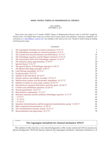
3The Arnold-Yost-Liouville theorem and KAM theory: 9/7/1711This means there are vectors e1 , . . . , en Rn such that(Γ x0 n m i e i m1 , . . . , m n Z),i 1and that ϕ establishes an isomorphismTn Rn /Γ x0 MG (c).This proves (2).Now we need to make the change-of-variables in (3); these new variables are called action-angle variables.First note that MG (c) is a Lagrangian submanifold, i.e. it’s half-dimensional and the restriction of ω to it is 0(it’s isotropic; an isotropic submanifold of R2n can be at most n-dimensional). This is because T MG (c) isspanned by { XGj }, and in (3.1), we proved ω ( XGj , XG ) { Gj , G } 0 for all j, .Consider the 1-formΘ : p j dq j .jThen,dΘ dp j dq j ω,jso restricted to MG (c), Θ is a closed 1-form.Let {γ j }nj 1 be a set of cycles whose homology classes generate H1 (MG (c)) H1 ( T n ) Zn . Then, theaction variables 1Ij (c) : Θ2π γjis independent of the choice of cycle representative of the homology class of γ j : if D is a 2-chain withej (a cobordism or homotopy from γ j to γej ), then by Stokes’ theorem. D γ j γ ˆˆΘ Θ dΘ 0 0.γjejγDDOne can show that the assignment (q, p) 7 (ϕ, I) is symplectic, where ϕ j is a variable parameterizing γ jand is called an angle variable (since it’s valued in S1 ). In these coordinates, H only depends on I, not ϕ, sodϕ H η(c)dt IdI H 0.dt ϕ Sometimes the entires of η(c) are irrational relative to each other. In this case you’ll get dense orbits inthe torus, corresponding to lines with irrational slope in R2n before quotienting by the lattice Γ x0 , and therewill not be n integrals of motion.Kolmogorov-Arnold-Moser (KAM) theory. More generally, if one doesn’t have complete integrability,one can make weaker but still interesting statements. For example, one can envision a problem whichis completely integrable in the absence of perturbations, and one can study what happens when thedependence on ϕ is small:H (ϕ, I) H0 (I) εH (ϕ, I).Some systems will lose integrability, though understanding the precise ways they do so is very hard. Sucha system is associated to a frequency vector η0 : η(I(t0 )) satisfying the Diophantine condition hη0 , ni 1hniτqfor all n Z for some τ 0. Here hxi : 1 x 2 is the Japanese bracket. This quantitatively captures thequalitative idea that “η0 is poorly approximated by rationals.”In this setup, there exists an invariant torus under the flow of H. The proof involves renormalizationgroup flow, though it was not originally discovered in those terms. It’s a kind of recursive proof style, and

M393C (Topics in Mathematical Physics) Lecture Notes12getting into the details would take a long time. It involves a great result called the shadowing lemma, whichdiscusses the dynamics of a pendulum.The pendulum has two equilibria: the bottom is stable (ϕ 0), and the top is unstable (both with novelocity). The phase space is two-dimensional, in ϕ and ϕ̇, and some trajectories are shown in Figure 1.The curves with singularities are called separatrices.Figure 1. The phase diagram of a pendulum. Source: https://physics.stackexchange.com/q/162577.Given a sequence of 0s and 1s, one may construct a parametric perturbation of the pendulum, regularlybumping it a small amount based on whether 0 or 1 is present.2. The shadowing lemma states that thesetrajectories uniformly approximate real trajectories. There’s a rich theory here: the proof is a fixed-pointargument, and there’s interesting geometry of the homoclinic points, where two trajectories meet. These tendto be concentrated near the unstable equilibrium.Quantum mechanics. Though quantum mechanics was discovered later than classical mechanics, it’sactually much more fundamental. This suggests that one can derive classical mechanics as some sort oflimit of quantum mechanics where Planck’s constant is small, and indeed we can do this. We’ll do this inthree ways.(1) The first is to use the Weiner transform to derive the Liouville equations from quantum mechanicsin a semiclassical limit.(2) The second case is to use a path integral to rediscover the principle of least action.(3) The third way is to use observables and something called the Ehrenfest theorem.Schrödinger discovered the Schrödinger equation, one of the cornerstones of quantum mechanics:ih̄ t ψ where ψ(t, x ) L2 andkψk2L2ˆ h̄2 ψ V ( x )ψ,2m ψ(t, x ) 2 dx 1,Schrödinger arrived at this equation by (somewhat heuristically) studying quantization. Electrons had beenobserved (by de Broglie) to sometimes behave as particles and sometimes behave as waves. If an electronbehaves like a particle, it has momentum h̄k, where k is something called a wave vector. If you look at it as awave, you get something like ih̄ e ikx , where P : ih̄ is called the momentum operator. The Schrödingerequation (a guess within his PhD thesis) replaced the true momentum in the HamiltonianH ( x, p) with the momentum operator ih̄ , giving is h̄2 .2TODO: did I get this right?1 2p V (x)2m

4The Arnold-Yost-Liouville theorem and KAM theory: 9/7/1713Lecture 4.The Schrödinger equation and the Wigner transform: 9/12/17Today we’re going to begin by asking, how does one derive (well, guess) the Schrödinger equation? Thisinvolves an interesting and relevant digression on the Hamilton-Jacobi equation.From the principle of least action, we know the Euler-Lagrange equations (1.1). Assume q0 (t) is asolution to these equations. Take a one-parameter variation (s, qs ) from (t0 , q0 ) to (t, q). The Hamiltonprincipal function isˆ (t,q)S(t, q) L(q(s), q̇(s)) ds.(t0 ,q0 )The variation with respect to q isˆ t L Lδq δq̇ dsδS q q̇t0 ˆ t L sδq ds q̇t0 Lδq q̇ Since p L q̇t.t0and δq(t0 ) 0, this is ( pδq)(t).Hence, p S qandL dS S Sq̇ j , dt t qjjso S L p j q̇ j tj H (q, q S).This is called the Hamilton-Jacobi equation.The link with the Schrödinger equation: let’s take for an ansatz that we have a wavefunctionψ(t, x ) a(t, x )e iS(t,x)/h̄ .This does not come entirely out of left field: if you want to exponentiate the action, you have to make itdimensionless, and that’s exactly what dividing by h̄ accomplishes. Then,h̄ S iS/h̄ae.h̄ t H (q, S)ψ O(h̄) 1 ( S)2 V ( x ) ψ O(h̄).2ih̄ t ψ ih̄ ȧe iS/h̄ Compare withh̄2h̄2i ae iS/h̄ S 22h̄ i Sh̄ 2 !ae iS./h̄ O(h̄)1( S2 ae iS/h̄ O(h̄).2Putting these together, we arrive atih̄ t ψ

which destroy photons. Thus imposing a fixed number of quantum particles is a constraint — and the theory which describes the quantum physics of arbitrary numbers of quantum particles, quantum field theory, was worked out a little later. In this case, the Hilbert space is a direct sum over the Hilbert subspace