WIXLIB

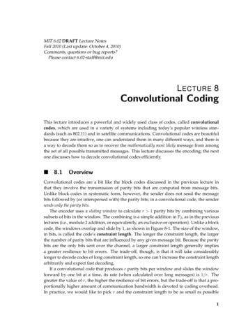
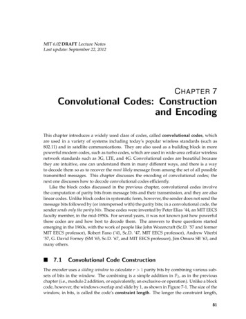
MIT 6.02 DRAFT Lecture NotesLast update: September 22, 2012C HAPTER 7Convolutional Codes: Constructionand EncodingThis chapter introduces a widely used class of codes, called convolutional codes, whichare used in a variety of systems including today’s popular wireless standards (such as802.11) and in satellite communications. They are also used as a building block in morepowerful modern codes, such as turbo codes, which are used in wide-area cellular wirelessnetwork standards such as 3G, LTE, and 4G. Convolutional codes are beautiful becausethey are intuitive, one can understand them in many different ways, and there is a wayto decode them so as to recover the most likely message from among the set of all possibletransmitted messages. This chapter discusses the encoding of convolutional codes; thenext one discusses how to decode convolutional codes efficiently.Like the block codes discussed in the previous chapter, convolutional codes involvethe computation of parity bits from message bits and their transmission, and they are alsolinear codes. Unlike block codes in systematic form, however, the sender does not send themessage bits followed by (or interspersed with) the parity bits; in a convolutional code, thesender sends only the parity bits. These codes were invented by Peter Elias ’44, an MIT EECSfaculty member, in the mid-1950s. For several years, it was not known just how powerfulthese codes are and how best to decode them. The answers to these questions startedemerging in the 1960s, with the work of people like John Wozencraft (Sc.D. ’57 and formerMIT EECS professor), Robert Fano (’41, Sc.D. ’47, MIT EECS professor), Andrew Viterbi’57, G. David Forney (SM ’65, Sc.D. ’67, and MIT EECS professor), Jim Omura SB ’63, andmany others. 7.1Convolutional Code ConstructionThe encoder uses a sliding window to calculate r 1 parity bits by combining various sub sets of bits in the window. The combining is a simple addition in F2 , as in the previouschapter (i.e., modulo 2 addition, or equivalently, an exclusive-or operation). Unlike a blockcode, however, the windows overlap and slide by 1, as shown in Figure 7-1. The size of thewindow, in bits, is called the code’s constraint length. The longer the constraint length,81

82CHAPTER 7. CONVOLUTIONAL CODES: CONSTRUCTION AND ENCODINGFigure 7-1: An example of a convolutional code with two parity bits per message bit and a constraint length(shown in the rectangular window) of three. I.e., r 2, K 3.the larger the number of parity bits that are influenced by any given message bit. Becausethe parity bits are the only bits sent over the channel, a larger constraint length generallyimplies a greater resilience to bit errors. The trade-off, though, is that it will take consider ably longer to decode codes of long constraint length (we will see in the next chapter thatthe complexity of decoding is exponential in the constraint length), so one cannot increasethe constraint length arbitrarily and expect fast decoding.If a convolutional code produces r parity bits per window and slides the window for ward by one bit at a time, its rate (when calculated over long messages) is 1/r. The greaterthe value of r, the higher the resilience of bit errors, but the trade-off is that a propor tionally higher amount of communication bandwidth is devoted to coding overhead. Inpractice, we would like to pick r and the constraint length to be as small as possible whileproviding a low enough resulting probability of a bit error.In 6.02, we will use K (upper case) to refer to the constraint length, a somewhat un fortunate choice because we have used k (lower case) in previous chapters to refer to thenumber of message bits that get encoded to produce coded bits. Although “L” might bea better way to refer to the constraint length, we’ll use K because many papers and doc uments in the field use K (in fact, many papers use k in lower case, which is especiallyconfusing). Because we will rarely refer to a “block” of size k while talking about convo lutional codes, we hope that this notation won’t cause confusion.Armed with this notation, we can describe the encoding process succinctly. The encoderlooks at K bits at a time and produces r parity bits according to carefully chosen functionsthat operate over various subsets of the K bits.1 One example is shown in Figure 7-1,which shows a scheme with K 3 and r 2 (the rate of this code, 1/r 1/2). The encoderspits out r bits, which are sent sequentially, slides the window by 1 to the right, and thenrepeats the process. That’s essentially it.At the transmitter, the two princial remaining details that we must describe are:1. What are good parity functions and how can we represent them conveniently?2. How can we implement the encoder efficiently?The rest of this chapter will discuss these issues, and also explain why these codes arecalled “convolutional”.1By convention, we will assume that each message has K - 1 “0” bits padded in front, so that the initialconditions work out properly.

83SECTION 7.2. PARITY EQUATIONS 7.2Parity EquationsThe example in Figure 7-1 shows one example of a set of parity equations, which governthe way in which parity bits are produced from the sequence of message bits, X. In thisexample, the equations are as follows (all additions are in F2 )):p0 [n] x[n] x[n - 1] x[n - 2]p1 [n] x[n] x[n - 1](7.1)The rate of this code is 1/2.An example of parity equations for a rate 1/3 code isp0 [n] x[n] x[n - 1] x[n - 2]p1 [n] x[n] x[n - 1]p2 [n] x[n] x[n - 2](7.2)In general, one can view each parity equation as being produced by combining the mes sage bits, X, and a generator polynomial, g. In the first example above, the generator poly nomial coefficients are (1, 1, 1) and (1, 1, 0), while in the second, they are (1, 1, 1), (1, 1, 0),and (1, 0, 1).We denote by gi the K-element generator polynomial for parity bit pi . We can thenwrite pi [n] as follows:k-1Xpi [n] (gi [j]x[n - j]).(7.3)j 0The form of the above equation is a convolution of g and x (modulo 2)—hence the term“convolutional code”. The number of generator polynomials is equal to the number ofgenerated parity bits, r, in each sliding window. The rate of the code is 1/r if the encoderslides the window one bit at a time. 7.2.1An ExampleLet’s consider the two generator polynomials of Equations 7.1 (Figure 7-1). Here, the gen erator polynomials areg0 1, 1, 1g1 1, 1, 0(7.4)If the message sequence, X [1, 0, 1, 1, . . .] (as usual, x[n] 0 8n 0), then the parity

84CHAPTER 7. CONVOLUTIONAL CODES: CONSTRUCTION AND ENCODINGbits from Equations 7.1 work out to bep0 [0] (1 0 0) 1p1 [0] (1 0) 1p0 [1] (0 1 0) 1p1 [1] (0 1) 1p0 [2] (1 0 1) 0p1 [2] (1 0) 1p0 [3] (1 1 0) 0(7.5)p1 [3] (1 1) 0.Therefore, the bits transmitted over the channel are [1, 1, 1, 1, 0, 0, 0, 0, . . .].There are several generator polynomials, but understanding how to construct goodones is outside the scope of 6.02. Some examples, found originally by J. Bussgang,2 areshown in Table 7-1.Constraint 11011110011001Table 7-1: Examples of generator polynomials for rate 1/2 convolutional codes with different constraintlengths. 7.3Two Views of the Convolutional EncoderWe now describe two views of the convolutional encoder, which we will find useful inbetter understanding convolutional codes and in implementing the encoding and decod ing procedures. The first view is in terms of shift registers, where one can construct themechanism using shift registers that are connected together. This view is useful in devel oping hardware encoders. The second is in terms of a state machine, which correspondsto a view of the encoder as a set of states with well-defined transitions between them. Thestate machine view will turn out to be extremely useful in figuring out how to decode a setof parity bits to reconstruct the original message bits.

SECTION 7.3. TWO VIEWS OF THE CONVOLUTIONAL ENCODER85Figure 7-2: Block diagram view of convolutional coding with shift registers. 7.3.1Shift-Register ViewFigure 7-2 shows the same encoder as Figure 7-1 and Equations (7.1) in the form of a blockdiagram made up of shift registers. The x[n - i] values (here there are two) are referred toas the state of the encoder. This block diagram takes message bits in one bit at a time, andspits out parity bits (two per input bit, in this case).Input message bits, x[n], arrive from the left. The block diagram calculates the paritybits using the incoming bits and the state of the encoder (the k - 1 previous bits; two in thisexample). After the r parity bits are produced, the state of the encoder shifts by 1, with x[n]taking the place of x[n - 1], x[n - 1] taking the place of x[n - 2], and so on, with x[n - K 1]being discarded. This block diagram is directly amenable to a hardware implementationusing shift registers. 7.3.2State-Machine ViewAnother useful view of convolutional codes is as a state machine, which is shown in Fig ure 7-3 for the same example that we have used throughout this chapter (Figure 7-1).An important point to note: the state machine for a convolutional code is identical forall codes with a given constraint length, K, and the number of states is always 2K-1 . Onlythe pi labels change depending on the number of generator polynomials and the valuesof their coefficients. Each state is labeled with x[n - 1]x[n - 2] . . . x[n - K 1]. Each arc islabeled with x[n]/p0 p1 . . . In this example, if the message is 101100, the transmitted bitsare 11 11 01 00 01 10.This state-machine view is an elegant way to explain what the transmitter does, and alsowhat the receiver ought to do to decode the message, as we now explain. The transmitterbegins in the initial state (labeled “STARTING STATE” in Figure 7-3) and processes themessage one bit at a time. For each message bit, it makes the state transition from thecurrent state to the new one depending on the value of the input bit, and sends the paritybits that are on the corresponding arc.The receiver, of course, does not have direct knowledge of the transmitter’s state transi 2Julian Bussgang, “Some Properties of Binary Convolutional Code Generators,” IEEE Transactions on In formation Theory, pp. 90–100, Jan. 1965. We will find in the next chapter that the (110, 111) code is actuallyinferior to another rate-1/2 K 3 code, (101, 111).