Transcription
MatConvNetConvolutional Neural Networks for MATLABAndrea VedaldiKarel LenciAnkush Gupta
iiAbstractMatConvNet is an implementation of Convolutional Neural Networks (CNNs)for MATLAB. The toolbox is designed with an emphasis on simplicity and flexibility.It exposes the building blocks of CNNs as easy-to-use MATLAB functions, providingroutines for computing linear convolutions with filter banks, feature pooling, and manymore. In this manner, MatConvNet allows fast prototyping of new CNN architectures; at the same time, it supports efficient computation on CPU and GPU allowingto train complex models on large datasets such as ImageNet ILSVRC. This documentprovides an overview of CNNs and how they are implemented in MatConvNet andgives the technical details of each computational block in the toolbox.
Contents1 Introduction to MatConvNet1.1 Getting started . . . . . . . .1.2 MatConvNet at a glance .1.3 Documentation and examples1.4 Speed . . . . . . . . . . . . .1.5 Acknowledgments . . . . . . .2 Neural Network Computations2.1 Overview . . . . . . . . . . . . . . . . . . . .2.2 Network structures . . . . . . . . . . . . . .2.2.1 Sequences . . . . . . . . . . . . . . .2.2.2 Directed acyclic graphs . . . . . . . .2.3 Computing derivatives with backpropagation2.3.1 Derivatives of tensor functions . . . .2.3.2 Derivatives of function compositions2.3.3 Backpropagation networks . . . . . .2.3.4 Backpropagation in DAGs . . . . . .2.3.5 DAG backpropagation networks . . .3 Wrappers and pre-trained models3.1 Wrappers . . . . . . . . . . . . .3.1.1 SimpleNN . . . . . . . . .3.1.2 DagNN . . . . . . . . . .3.2 Pre-trained models . . . . . . . .3.3 Learning models . . . . . . . . . .3.4 Running large scale experiments .3.5 Reading images . . . . . . . . . .124567.99101011121213141518.21212121222323234 Computational blocks4.1 Convolution . . . . . . . . . . . . . . .4.2 Convolution transpose (deconvolution)4.3 Spatial pooling . . . . . . . . . . . . .4.4 Activation functions . . . . . . . . . .4.5 Spatial bilinear resampling . . . . . . .4.6 Region of interest pooling . . . . . . .27272931323232.iii
ivCONTENTS4.74.84.9Normalization . . . . . . . . . . . . . . . . .4.7.1 Local response normalization (LRN)4.7.2 Batch normalization . . . . . . . . .4.7.3 Spatial normalization . . . . . . . . .4.7.4 Softmax . . . . . . . . . . . . . . . .Categorical losses . . . . . . . . . . . . . . .4.8.1 Classification losses . . . . . . . . . .4.8.2 Attribute losses . . . . . . . . . . . .Comparisons . . . . . . . . . . . . . . . . . .4.9.1 p-distance . . . . . . . . . . . . . . .5 Geometry5.1 Preliminaries . . . . . . . .5.2 Simple filters . . . . . . . .5.2.1 Pooling in Caffe . . .5.3 Convolution transpose . . .5.4 Transposing receptive fields5.5 Composing receptive fields .5.6 Overlaying receptive fields .6 Implementation details6.1 Convolution . . . . . . . . . . . . . . . . . .6.2 Convolution transpose . . . . . . . . . . . .6.3 Spatial pooling . . . . . . . . . . . . . . . .6.4 Activation functions . . . . . . . . . . . . .6.4.1 ReLU . . . . . . . . . . . . . . . . .6.4.2 Sigmoid . . . . . . . . . . . . . . . .6.5 Spatial bilinear resampling . . . . . . . . . .6.6 Normalization . . . . . . . . . . . . . . . . .6.6.1 Local response normalization (LRN)6.6.2 Batch normalization . . . . . . . . .6.6.3 Spatial normalization . . . . . . . . .6.6.4 Softmax . . . . . . . . . . . . . . . .6.7 Categorical losses . . . . . . . . . . . . . . .6.7.1 Classification losses . . . . . . . . . .6.7.2 Attribute losses . . . . . . . . . . . .6.8 Comparisons . . . . . . . . . . . . . . . . . .6.8.1 p-distance . . . . . . . . . . . . . . .6.9 Other implementation details . . . . . . . .6.9.1 Normal sampler . . . . . . . . . . . .6.9.2 Euclid’s algorithm . . . . . . . . . 4.45454647474748484848495050515151525252525455
Chapter 1Introduction to MatConvNetMatConvNet is a MATLAB toolbox implementing Convolutional Neural Networks (CNN)for computer vision applications. Since the breakthrough work of [8], CNNs have had amajor impact in computer vision, and image understanding in particular, essentially replacingtraditional image representations such as the ones implemented in our own VLFeat [13] opensource library.While most CNNs are obtained by composing simple linear and non-linear filtering operations such as convolution and rectification, their implementation is far from trivial. Thereason is that CNNs need to be learned from vast amounts of data, often millions of images,requiring very efficient implementations. As most CNN libraries, MatConvNet achievesthis by using a variety of optimizations and, chiefly, by supporting computations on GPUs.Numerous other machine learning, deep learning, and CNN open source libraries exist.To cite some of the most popular ones: CudaConvNet,1 Torch,2 Theano,3 and Caffe4 . Manyof these libraries are well supported, with dozens of active contributors and large user bases.Therefore, why creating yet another library?The key motivation for developing MatConvNet was to provide an environment particularly friendly and efficient for researchers to use in their investigations.5 MatConvNetachieves this by its deep integration in the MATLAB environment, which is one of the mostpopular development environments in computer vision research as well as in many other areas.In particular, MatConvNet exposes as simple MATLAB commands CNN building blockssuch as convolution, normalisation and pooling (chapter 4); these can then be combined andextended with ease to create CNN architectures. While many of such blocks use optimisedCPU and GPU implementations written in C and CUDA (section section 1.4), MATLABnative support for GPU computation means that it is often possible to write new blocksin MATLAB directly while maintaining computational efficiency. Compared to writing newCNN components using lower level languages, this is an important simplification that cansignificantly accelerate testing new ideas. Using MATLAB also provides a bridge p://cilvr.nyu.edu/doku.php?id /4http://caffe.berkeleyvision.org25While from a user perspective MatConvNet currently relies on MATLAB, the library is being developed with a clean separation between MATLAB code and the C and CUDA core; therefore, in the futurethe library may be extended to allow processing convolutional networks independently of MATLAB.1
2CHAPTER 1. INTRODUCTION TO MATCONVNETother areas; for instance, MatConvNet was recently used by the University of Arizona inplanetary science, as summarised in this NVIDIA blogpost.6MatConvNet can learn large CNN models such AlexNet [8] and the very deep networksof [11] from millions of images. Pre-trained versions of several of these powerful models canbe downloaded from the MatConvNet home page7 . While powerful, MatConvNet remains simple to use and install. The implementation is fully self-contained, requiring onlyMATLAB and a compatible C compiler (using the GPU code requires the freely-availableCUDA DevKit and a suitable NVIDIA GPU). As demonstrated in fig. 1.1 and section 1.1,it is possible to download, compile, and install MatConvNet using three MATLAB commands. Several fully-functional examples demonstrating how small and large networks canbe learned are included. Importantly, several standard pre-trained network can be immediately downloaded and used in applications. A manual with a complete technical descriptionof the toolbox is maintained along with the toolbox.8 These features make MatConvNetuseful in an educational context too.9MatConvNet is open-source released under a BSD-like license. It can be downloadedfrom http://www.vlfeat.org/matconvnet as well as from GitHub.10 .1.1Getting startedMatConvNet is simple to install and use. fig. 1.1 provides a complete example that classifies an image using a latest-generation deep convolutional neural network. The exampleincludes downloading MatConvNet, compiling the package, downloading a pre-trained CNNmodel, and evaluating the latter on one of MATLAB’s stock images.The key command in this example is vl simplenn, a wrapper that takes as input theCNN net and the pre-processed image im and produces as output a structure res of results.This particular wrapper can be used to model networks that have a simple structure, namelya chain of operations. Examining the code of vl simplenn (edit vl simplenn in MatConvNet) we note that the wrapper transforms the data sequentially, applying a number ofMATLAB functions as specified by the network configuration. These function, discussed indetail in chapter 4, are called “building blocks” and constitute the backbone of MatConvNet.While most blocks implement simple operations, what makes them non trivial is theirefficiency (section 1.4) as well as support for backpropagation (section 2.3) to allow learningCNNs. Next, we demonstrate how to use one of such building blocks directly. For the sake ofthe example, consider convolving an image with a bank of linear filters. Start by reading animage in MATLAB, say using im single(imread('peppers.png')), obtaining a H W Darray im, where D 3 is the number of colour channels in the image. Then create a bankof K 16 random filters of size 3 3 using f randn(3,3,3,16,'single'). Finally, convolve /matconvnet/matconvnet-manual.pdf9An example laboratory experience based on MatConvNet can be downloaded from http://www.robots.ox.ac.uk/ com/matconvnet7
1.1. GETTING STARTED3% install and compile MatConvNet (run load/' .'matconvnet 1.0 beta25.tar.gz']) ;cd matconvnet 1.0 beta25run matlab/vl compilenn% download a pre trained CNN from the web (run odels/imagenet vgg f.mat', .'imagenet vgg f.mat') ;% setup MatConvNetrun matlab/vl setupnn% load the pre trained CNNnet load('imagenet vgg f.mat') ;% load and preprocess an imageim imread('peppers.png') ;im imresize(single(im), net.meta.normalization.imageSize(1:2)) ;im im net.meta.normalization.averageImage ;% run the CNNres vl simplenn(net, im ) ;bell pepper (946), score 0.704% show the classification resultscores squeeze(gather(res(end).x)) ;[bestScore, best] max(scores) ;figure(1) ; clf ; imagesc(im) ;title(sprintf('%s (%d), score %.3f',.net.classes.description{best}, best, bestScore)) ;Figure 1.1: A complete example including download, installing, compiling and running MatConvNet to classify one of MATLAB stock images using a large CNN pre-trained onImageNet.
4CHAPTER 1. INTRODUCTION TO MATCONVNETimage with the filters by using the command y vl nnconv(x,f,[]). This results in an arrayy with K channels, one for each of the K filters in the bank.While users are encouraged to make use of the blocks directly to create new architectures,MATLAB provides wrappers such as vl simplenn for standard CNN architectures such asAlexNet [8] or Network-in-Network [9]. Furthermore, the library provides numerous examples(in the examples/ subdirectory), including code to learn a variety of models on the MNIST,CIFAR, and ImageNet datasets. All these examples use the examples/cnn train trainingcode, which is an implementation of stochastic gradient descent (section 3.3). While thistraining code is perfectly serviceable and quite flexible, it remains in the examples/ subdirectory as it is somewhat problem-specific. Users are welcome to implement their optimisers.1.2MatConvNet at a glanceMatConvNet has a simple design philosophy. Rather than wrapping CNNs around complexlayers of software, it exposes simple functions to compute CNN building blocks, such as linearconvolution and ReLU operators, directly as MATLAB commands. These building blocks areeasy to combine into complete CNNs and can be used to implement sophisticated learningalgorithms. While several real-world examples of small and large CNN architectures andtraining routines are provided, it is always possible to go back to the basics and build yourown, using the efficiency of MATLAB in prototyping. Often no C coding is required at allto try new architectures. As such, MatConvNet is an ideal playground for research incomputer vision and CNNs.MatConvNet contains the following elements: CNN computational blocks. A set of optimized routines computing fundamentalbuilding blocks of a CNN. For example, a convolution block is implemented byy vl nnconv(x,f,b) where x is an image, f a filter bank, and b a vector of biases (section 4.1). The derivatives are computed as [dzdx,dzdf,dzdb] vl nnconv(x,f,b,dzdy)where dzdy is the derivative of the CNN output w.r.t y (section 4.1). chapter 4 describes all the blocks in detail. CNN wrappers. MatConvNet provides a simple wrapper, suitably invoked byvl simplenn, that implements a CNN with a linear topology (a chain of blocks). It alsoprovides a much more flexible wrapper supporting networks with arbitrary topologies,encapsulated in the dagnn.DagNN MATLAB class. Example applications. MatConvNet provides several examples of learning CNNs withstochastic gradient descent and CPU or GPU, on MNIST, CIFAR10, and ImageNetdata. Pre-trained models. MatConvNet provides several state-of-the-art pre-trained CNNmodels that can be used off-the-shelf, either to classify images or to produce imageencodings in the spirit of Caffe or DeCAF.
1.3. DOCUMENTATION AND EXAMPLES50.9dropout top-1 valdropout top-5 valbnorm top-1 valbnorm top-5 val0.80.70.60.50.40.30.20102030405060epochFigure 1.2: Training AlexNet on ImageNet ILSVRC: dropout vs batch normalisation.1.3Documentation and examplesThere are three main sources of information about MatConvNet. First, the website contains descriptions of all the functions and several examples and tutorials.11 Second, thereis a PDF manual containing a great deal of technical details about the toolbox, includingdetailed mathematical descriptions of the building blocks. Third, MatConvNet ships withseveral examples (section 1.1).Most examples are fully self-contained. For example, in order to run the MNIST example,it suffices to point MATLAB to the MatConvNet root directory and type addpath examples followed by cnn mnist. Due to the problem size, the ImageNet ILSVRC examplerequires some more preparation, including downloading and preprocessing the images (usingthe bundled script utils/preprocess imagenet.sh). Several advanced examples are includedas well. For example, fig. 1.2 illustrates the top-1 and top-5 validation errors as a modelsimilar to AlexNet [8] is trained using either standard dropout regularisation or the recentbatch normalisation technique of [4]. The latter is shown to converge in about one third ofthe epochs (passes through the training data) required by the former.The MatConvNet website contains also numerous pre-trained models, i.e. large CNNstrained on ImageNet ILSVRC that can be downloaded and used as a starting point for manyother problems [1]. These include: AlexNet [8], VGG-S, VGG-M, VGG-S [1], and VGG-VD16, and VGG-VD-19 [12]. The example code of fig. 1.1 shows how one such model can beused in a few lines of MATLAB code.11See also http://www.robots.ox.ac.uk/ vgg/practicals/cnn/index.html.
6CHAPTER 1. INTRODUCTION TO MATCONVNETmodelbatch G-VD-1924CPU GPU22.1 192.421.4 211.47.8 120.016.5Table 1.1: ImageNet training speed (images/s).1.4SpeedEfficiency is very important for working with CNNs. MatConvNet supports using NVIDIAGPUs as it includes CUDA implementations of all algorithms (or relies on MATLAB CUDAsupport).To use the GPU (provided that suitable hardware is available and the toolbox has beencompiled with GPU support), one simply converts the arguments to gpuArrays in MATLAB,as in y vl nnconv(gpuArray(x), gpuArray(w), []). In this manner, switching between CPUand GPU is fully transparent. Note that MatConvNet can also make use of the NVIDIACuDNN library with significant speed and space benefits.Next we evaluate the performance of MatConvNet when training large architectureson the ImageNet ILSVRC 2012 challenge data [2]. The test machine is a Dell server withtwo Intel Xeon CPU E5-2667 v2 clocked at 3.30 GHz (each CPU has eight cores), 256 GBof RAM, and four NVIDIA Titan Black GPUs (only one of which is used unless otherwisenoted). Experiments use MatConvNet beta12, CuDNN v2, and MATLAB R2015a. Thedata is preprocessed to avoid rescaling images on the fly in MATLAB and stored in a RAMdisk for faster access. The code uses the vl imreadjpeg command to read large batches ofJPEG images from disk in a number of separate threads. The driver examples/cnn imagenet.mis used in all experiments.We train the models discussed in section 1.3 on ImageNet ILSVRC. table 1.1 reportsthe training speed as number of images per second processed by stochastic gradient descent.AlexNet trains at about 264 images/s with CuDNN, which is about 40% faster than thevanilla GPU implementation (using CuBLAS) and more than 10 times faster than using theCPUs. Furthermore, we note that, despite MATLAB overhead, the implementation speed iscomparable to Caffe (they report 253 images/s with CuDNN and a Titan – a slightly slowerGPU than the Titan Black used here). Note also that, as the model grows in size, the size ofa SGD batch must be decreased (to fit in the GPU memory), increasing the overhead impactsomewhat.table 1.2 reports the speed on VGG-VD-16, a very large model, using multiple GPUs. Inthis case, the batch size is set to 264 images. These are further divided in sub-batches of 22images each to fit in the GPU memory; the latter are then distributed among one to fourGPUs on the same machine. While there is a substantial communication overhead, trainingspeed increases from 20 images/s to 45. Addressing this overhead is one of the medium termgoals of the library.
1.5. ACKNOWLEDGMENTSnum GPUsVGG-VD-16 speed7120.0222.20338.18444.8Table 1.2: Multiple GPU speed (images/s).1.5AcknowledgmentsMatConvNet is a community project, and as such acknowledgements go to all contributors.We kindly thank NVIDIA supporting this project by providing us with top-of-the-line GPUsand MathWorks for ongoing discussion on how to improve the library.The implementation of several CNN computations in this library are inspired by the Caffelibrary [6] (however, Caffe is not a dependency). Several of the example networks have beentrained by Karen Simonyan as part of [1] and [12].
Chapter 2Neural Network ComputationsThis chapter provides a brief introduction to the computational aspects of neural networks,and convolutional neural networks in particular, emphasizing the concepts required to understand and use MatConvNet.2.1OverviewA Neural Network (NN) is a function g mapping data x, for example an image, to an outputvector y, for example an image label. The function g fL · · · f1 is the compositionof a sequence of simpler functions fl , which are called computational blocks or layers. Letx1 , x2 , . . . , xL be the outputs of each layer in the network, and let x0 x denote the networkinput. Each intermediate output xl fl (xl 1 ; wl ) is computed from the previous output xl 1by applying the function fl with parameters wl .In a Convolutional Neural Network (CNN), the data has a spatial structure: each xl Hl Wl ClRis a 3D array or tensor where the first two dimensions Hl (height) and Wl (width)are interpreted as spatial dimensions. The third dimension Cl is instead interpreted asthe number of feature channels. Hence, the tensor xl represents a Hl Wl field of Cl dimensional feature vectors, one for each spatial location. A fourth dimension Nl in thetensor spans multiple data samples packed in a single batch for efficiency parallel processing.The number of data samples Nl in a batch is called the batch cardinality. The network iscalled convolutional because the functions fl are local and translation invariant operators(i.e. non-linear filters) like linear convolution.It is also possible to conceive CNNs with more than two spatial dimensions, where theadditional dimensions may represent volume or time. In fact, there are little a-priori restrictions on the format of data in neural networks in general. Many useful NNs contain amixture of convolutional layers together with layer that process other data types such as textstrings, or perform other operations that do not strictly conform to the CNN assumptions.MatConvNet includes a variety of layers, contained in the matlab/ directory, suchas vl nnconv (convolution), vl nnconvt (convolution transpose or deconvolution), vl nnpool(max and average pooling), vl nnrelu (ReLU activation), vl nnsigmoid (sigmoid activation),vl nnsoftmax (softmax operator), vl nnloss (classification log-loss), vl nnbnorm (batch normalization), vl nnspnorm (spatial normalization), vl nnnormalize (local response normal9
10CHAPTER 2. NEURAL NETWORK COMPUTATIONSization – LRN), or vl nnpdist (p-distance). There are enough layers to implement manyinteresting state-of-the-art networks out of the box, or even import them from other toolboxes such as Caffe.NNs are often used as classifiers or regressors. In the example of fig. 1.1, the outputŷ f (x) is a vector of probabilities, one for each of a 1,000 possible image labels (dog, cat,trilobite, .). If y is the true label of image x, we can measure the CNN performance by aloss function y (ŷ) R which assigns a penalty to classification errors. The CNN parameterscan then be tuned or learned to minimize this loss averaged over a large dataset of labelledexample images.Learning generally uses a variant of stochastic gradient descent (SGD). While this is anefficient method (for this type of problems), networks may contain several million parametersand need to be trained on millions of images; thus, efficiency is a paramount in MATLABdesign, as further discussed in section 1.4. SGD also requires to compute the CNN derivatives,as explained in the next section.2.2Network structuresIn the simplest case, layers in a NN are arranged in a sequence; however, more complexinterconnections are possible as well, and in fact very useful in many cases. This sectiondiscusses such configurations and introduces a graphical notation to visualize them.2.2.1SequencesStart by considering a computational block f in the network. This can be representedschematically as a box receiving data x and parameters w as inputs and producing data yas output:xyfwAs seen above, in the simplest case blocks are chained in a sequence f1 f2 · · · fLyielding the structure:x0f1w1x1f2w2x2.xL 1fLxLwLGiven an input x0 , evaluating the network is a simple matter of evaluating all the blocksfrom left to right, which defines a composite function xL f (x0 ; w1 , . . . , wL ).
2.2. NETWORK re 2.1: Example DAG.2.2.2Directed acyclic graphsOne is not limited to chaining layers one after another. In fact, the only requirement forevaluating a NN is that, when a layer has to be evaluated, all its input have been evaluatedprior to it. This is possible exactly when the interconnections between layers form a directedacyclic graph, or DAG for short.In order to visualize DAGs, it is useful to introduce additional nodes for the networkvariables, as in the example of Fig. 2.1. Here boxes denote functions and circles denotevariables (parameters are treated as a special kind of variables). In the example, x0 and x4are the inputs of the CNN and x6 and x7 the outputs. Functions can take any number ofinputs (e.g. f3 and f5 take two) and have any number of outputs (e.g. f4 has two). Thereare a few noteworthy properties of this graph:1. The graph is bipartite, in the sense that arrows always go from boxes to circles andfrom circles to boxes.2. Functions can have any number of inputs or outputs; variables and parameters canhave an arbitrary number of outputs (a parameter with more of one output is sharedbetween different layers); variables have at most one input and parameters none.3. Variables with no incoming arrows and parameters are not computed by the network,but must be set prior to evaluation, i.e. they are inputs. Any variable (or even parameter) may be used as output, although these are usually the variables with no outgoingarrows.
12CHAPTER 2. NEURAL NETWORK COMPUTATIONS4. Since the graph is acyclic, the CNN can be evaluated by sorting the functions andcomputing them one after another (in the example, evaluating the functions in theorder f1 , f2 , f3 , f4 , f5 would work).2.3Computing derivatives with backpropagationLearning a NN requires computing the derivative of the loss with respect to the networkparameters. Derivatives are computed using an algorithm called backpropagation, which isa memory-efficient implementation of the chain rule for derivatives. First, we discuss thederivatives of a single layer, and then of a whole network.2.3.1Derivatives of tensor functionsIn a CNN, a layer is a function y f (x) where both input x RH W C and output000y RH W C are tensors. The derivative of the function f contains the derivative ofeach output component yi0 j 0 k0 with respect to each input component xijk , for a total ofH 0 W 0 C 0 H W C elements naturally arranged in a 6D tensor. Instead of expressingderivatives as tensors, it is often useful to switch to a matrix notation by stacking the inputand output tensors into vectors. This is done by the vec operator, which visits each elementof a tensor in lexicographical order and produces a vector: x111 x211 . . . vec x xH11 . x121 . . xHW CBy stacking both input and output, each layer f can be seen reinterpreted as vector functionvec f , whose derivative is the conventional Jacobian matrix: y111 y111 y111 y111 y111. x211 xH11 x121 xHW C x111 y211 y211 y211 y211211 x111 . . . x yHW x211 xH11 x121C . . d vec f yH 0 11 yH 0 11 yH 0 11 yH 0 11 yH 0 11 . x211 xH11 x121 xHW C d(vec x) x111 y121 y121 y121 y121121 x . . . x yHW x211 xH11 x121111C . . yH 0 W 0 C 0 yH 0 W 0 C 0 yH 0 W 0 C 0 yH 0 W 0 C 0 yH 0 W 0 C 0. . . xHW C x111 x211 xH11 x121This notation for the derivatives of tensor functions is taken from [7] and is used throughoutthis document.
2.3. COMPUTING DERIVATIVES WITH BACKPROPAGATION13While it is easy to express the derivatives of tensor functions as matrices, these matricesare in general extremely large. Even for moderate data sizes (e.g. H H 0 W W 0 32 and C C 0 128), there are H 0 W 0 C 0 HW C 17 109 elements in the Jacobian.Storing that requires 68 GB of space in single precision. The purpose of the backpropagationalgorithm is to compute the derivatives required for learning without incurring this hugememory cost.2.3.2Derivatives of function compositionsIn order to understand backpropagation, consider first a simple CNN terminating in a lossfunction fL y :x0f1x1w1f2w2x2.xL 1fLxl RwLThe goal is to compute the gradient of the loss value xL (output) with respect to each networkparameter wl :ddf [fL (·; wL ) . f2 (·; w2 ) f1 (x0 ; w1 )] . d(vec wl )d(vec wl ) By applying the chain rule and by using the matrix notation introduced above, the derivativecan be written asdfd vec fL (xL 1 ; wL )d vec fl 1 (xl ; wl 1 ) d vec fl (xl 1 ; wl ) ··· d(vec wl )d(vec xL 1 )d(vec xl ) d(vec wl )(2.1)where the derivatives are computed at the working point determined by the input x0 and thecurrent value of the parameters.Note that, since the network output xl is a scalar quantity, the target derivativedf /d(vec wl ) has the same number of elements of the parameter vector wl , which is moderate. However, the intermediate Jacobian factors have, as seen above, an unmanageable size.In order to avoid computing these factor explicitly, we can proceed as follows.Start by multiplying the output of the last layer by a tensor pL 1 (note that this tensoris a scalar just like the variable xL ):pL d vec fl 1 (xl ; wl 1 ) d vec fl (xl 1 ; wl )dfd vec fL (xL 1 ; wL ) pL ··· d(vec wl )d(vec xL 1 )d(vec xl ) d(vec wl ) {z}(vec pL 1 ) (vec pL 1 ) · · · d vec fl 1 (xl ; wl 1 ) d vec fl (xl 1 ; wl ) d(vec xl ) d(vec wl )In the sec
MatConvNet is an implementation of Convolutional Neural Networks (CNNs) for MATLAB. The toolbox is designed with an emphasis on simplicity and exibility. It exposes the building blocks of CNNs as easy-to-use MATLAB functions, providing routines for computing linear conv