WIXLIB

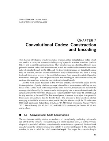
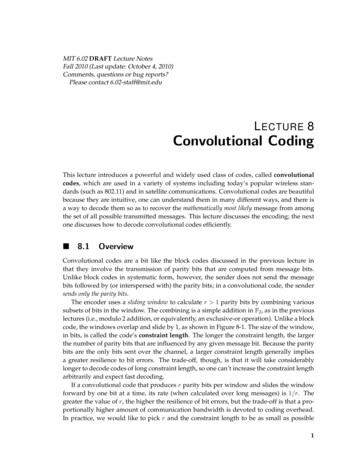
MIT 6.02 DRAFT Lecture NotesFall 2010 (Last update: October 4, 2010)Comments, questions or bug reports?Please contact 6.02-staff@mit.eduL ECTURE 8Convolutional CodingThis lecture introduces a powerful and widely used class of codes, called convolutionalcodes, which are used in a variety of systems including today’s popular wireless standards (such as 802.11) and in satellite communications. Convolutional codes are beautifulbecause they are intuitive, one can understand them in many different ways, and there isa way to decode them so as to recover the mathematically most likely message from amongthe set of all possible transmitted messages. This lecture discusses the encoding; the nextone discusses how to decode convolutional codes efficiently. 8.1OverviewConvolutional codes are a bit like the block codes discussed in the previous lecture inthat they involve the transmission of parity bits that are computed from message bits.Unlike block codes in systematic form, however, the sender does not send the messagebits followed by (or interspersed with) the parity bits; in a convolutional code, the sendersends only the parity bits.The encoder uses a sliding window to calculate r 1 parity bits by combining varioussubsets of bits in the window. The combining is a simple addition in F2 , as in the previouslectures (i.e., modulo 2 addition, or equivalently, an exclusive-or operation). Unlike a blockcode, the windows overlap and slide by 1, as shown in Figure 8-1. The size of the window,in bits, is called the code’s constraint length. The longer the constraint length, the largerthe number of parity bits that are influenced by any given message bit. Because the paritybits are the only bits sent over the channel, a larger constraint length generally impliesa greater resilience to bit errors. The trade-off, though, is that it will take considerablylonger to decode codes of long constraint length, so one can’t increase the constraint lengtharbitrarily and expect fast decoding.If a convolutional code that produces r parity bits per window and slides the windowforward by one bit at a time, its rate (when calculated over long messages) is 1/r. Thegreater the value of r, the higher the resilience of bit errors, but the trade-off is that a proportionally higher amount of communication bandwidth is devoted to coding overhead.In practice, we would like to pick r and the constraint length to be as small as possible1

2LECTURE 8. CONVOLUTIONAL CODINGFigure 8-1: An example of a convolutional code with two parity bits per message bit (r 2) and constraintlength (shown in the rectangular window) K 3.while providing a low enough resulting probability of a bit error.In 6.02, we will use K (upper case) to refer to the constraint length, a somewhat unfortunate choice because we have used k (lower case) in previous lectures to refer to thenumber of message bits that get encoded to produce coded bits. Although “L” might bea better way to refer to the constraint length, we’ll use K because many papers and documents in the field use K (in fact, most use k in lower case, which is especially confusing).Because we will rarely refer to a “block” of size k while talking about convolutional codes,we hope that this notation won’t cause confusion.Armed with this notation, we can describe the encoding process succinctly. The encoderlooks at K bits at a time and produces r parity bits according to carefully chosen functionsthat operate over various subsets of the K bits.1 One example is shown in Figure 8-1,which shows a scheme with K 3 and r 2 (the rate of this code, 1/r 1/2). The encoderspits out r bits, which are sent sequentially, slides the window by 1 to the right, and thenrepeats the process. That’s essentially it.At the transmitter, the only remaining details that we have to worry about now are:1. What are good parity functions and how can we represent them conveniently?2. How can we implement the encoder efficiently?The rest of this lecture will discuss these issues, and also explain why these codes arecalled “convolutional”. 8.2Parity EquationsThe example in Figure 8-1 shows one example of a set of parity equations, which governthe way in which parity bits are produced from the sequence of message bits, X. In thisexample, the equations are as follows (all additions are in F2 )):p0 [n] x[n] x[n 1] x[n 2]p1 [n] x[n] x[n 1]1(8.1)By convention, we will assume that each message has K 1 “0” bits padded in front, so that the initialconditions work out properly.

3SECTION 8.2. PARITY EQUATIONSAn example of parity equations for a rate 1/3 code isp0 [n] x[n] x[n 1] x[n 2]p1 [n] x[n] x[n 1]p2 [n] x[n] x[n 2](8.2)In general, one can view each parity equation as being produced by composing the message bits, X, and a generator polynomial, g. In the first example above, the generator polynomial coefficients are (1, 1, 1) and (1, 1, 0), while in the second, they are (1, 1, 1), (1, 1, 0),and (1, 0, 1).We denote by gi the K-element generator polynomial for parity bit pi . We can thenwrite pi as follows:k 1 pi [n] (gi [j]x[n j]) mod 2.(8.3)j 0The form of the above equation is a convolution of g and x—hence the term “convolutional code”. The number of generator polynomials is equal to the number of generatedparity bits, r, in each sliding window. 8.2.1An ExampleLet’s consider the two generator polynomials of Equations 8.1 (Figure 8-1). Here, the generator polynomials areg0 1, 1, 1g1 1, 1, 0(8.4)If the message sequence, X [1, 0, 1, 1, . . .] (as usual, x[n] 0 n 0), then the paritybits from Equations 8.1 work out to bep0 [0] (1 0 0) 1p1 [0] (1 0) 1p0 [1] (0 1 0) 1p1 [1] (0 1) 1p0 [2] (1 0 1) 0p1 [2] (1 0) 1p0 [3] (1 1 0) 0p1 [3] (1 1) 0.(8.5)Therefore, the parity bits sent over the channel are [1, 1, 1, 1, 0, 0, 0, 0, . . .].There are several generator polynomials, but understanding how to construct goodones is outside the scope of 6.02. Some examples (found by J. Busgang) are shown inTable 8-1.

4LECTURE 8. CONVOLUTIONAL CODINGConstraint 11011110011001Table 8-1: Examples of generator polynomials for rate 1/2 convolutional codes with different constraintlengths.Figure 8-2: Block diagram view of convolutional coding with shift registers. 8.3Two Views of the Convolutional EncoderWe now describe two views of the convolutional encoder, which we will find useful inbetter understanding convolutional codes and in implementing the encoding and decoding procedures. The first view is in terms of a block diagram, where one can constructthe mechanism using shift registers that are connected together. The second is in terms ofa state machine, which corresponds to a view of the encoder as a set of states with welldefined transitions between them. The state machine view will turn out to be extremelyuseful in figuring out how to decode a set of parity bits to reconstruct the original messagebits. 8.3.1Block Diagram ViewFigure 8-2 shows the same encoder as Figure 8-1 and Equations (8.1) in the form of a blockdiagram. The x[n i] values (here there are two) are referred to as the state of the encoder.The way to think of this block diagram is as a “black box” that takes message bits in andspits out parity bits.Input message bits, x[n], arrive on the wire from the left. The box calculates the paritybits using the incoming bits and the state of the encoder (the k 1 previous bits; 2 in thisexample). After the r parity bits are produced, the state of the encoder shifts by 1, with x[n]

SECTION 8.3. TWO VIEWS OF THE CONVOLUTIONAL ENCODER5Figure 8-3: State machine view of convolutional coding.taking the place of x[n 1], x[n 1] taking the place of x[n 2], and so on, with x[n K 1]being discarded. This block diagram is directly amenable to a hardware implementationusing shift registers. 8.3.2State Machine ViewAnother useful view of convolutional codes is as a state machine, which is shown in Figure 8-3 for the same example that we have used throughout this lecture (Figure 8-1).The state machine for a convolutional code is identical for all codes with a given constraint length, K, and the number of states is always 2K 1 . Only the pi labels change depending on the number of generator polynomials and the values of their coefficients. Eachstate is labeled with x[n 1]x[n 2] . . . x[n K 1]. Each arc is labeled with x[n]/p0 p1 . . .In this example, if the message is 101100, the transmitted bits are 11 11 01 00 01 10.This state machine view is an elegant way to explain what the transmitter does, and alsowhat the receiver ought to do to decode the message, as we now explain. The transmitterbegins in the initial state (labeled “STARTING STATE” in Figure 8-3) and processes themessage one bit at a time. For each message bit, it makes the state transition from thecurrent state to the new one depending on the value of the input bit, and sends the paritybits that are on the corresponding arc.The receiver, of course, does not have direct knowledge of the transmitter’s state transitions. It only sees the received sequence of parity bits, with possible corruptions. Its task isto determine the best possible sequence of transmitter states that could have producedthe parity bit sequence. This task is called decoding, which we will introduce next, andthen study in more detail in the next lecture.