Transcription
Chapter 3The Magnetic Field of the EarthIntroductionStudies of the geomagnetic field have a long history, in particular because of its importance fornavigation. The geomagnetic field and its variations over time are our most direct ways to studythe dynamics of the core. The variations with time of the geomagnetic field, the secular variations,are the basis for the science of paleomagnetism, and several major discoveries in the late fiftiesgave important new impulses to the concept of plate tectonics. Magnetism also plays a major rolein exploration geophysics in the search for ore deposits.Because of its use as a navigation tool, the study of the magnetic field has a very long history, and probably goes back to the 12 C when it was first exploited by the Chinese. It was not until 1600that Gilbert postulated that the Earth is, in fact, a gigantic magnet. The origin of the Earth’s fieldhas, however, remained enigmatic for another 300 years after Gilbert’s manifesto ’De Magnete’.It was also known early on that the field was not constant in time, and the secular variation is wellrecorded so that a very useful historical record of the variations in strength and, in particular, indirection is available for research. The first (known) map of declination was published by Halley(yes, the one of the comet) in 1701 (the ’chart of the lines of equal magnetic variation’, also knownas the ’Tabula Nautica’).The source of the main field and the cause of the secular variation remained a mystery sincethe rapid fluctuations seemed to be at odds with the rigidity of the Earth, and until early thiscentury an external origin of the field was seriously considered. In a breakthrough (1838) Gausswas able to prove that almost the entire field has to be of internal origin. Gauss used sphericalharmonics and showed that the coefficients of the field expansion, which he determined by fittingthe surface harmonics to the available magnetic data at that time (a small number of magnetic fieldmeasurements at intervals of about 30 along several parallels - lines of constant latitude), werealmost identical to the coefficients for a field due to a magnetized sphere or to a dipole. In fact,he also showed from a spectral analysis that the best fit to the observed field was obtained if thedipole was not purely axial but made an angle of about 11 with the Earth’s rotation axis.An outstanding issue remained: what causes the internal field? It was clear that the temperatures inthe interior of the Earth are probably much too high to sustain permanent magnetization. A majorleap in the understanding of the origin of the field came in the first decade of this century whenOldham (1906) and Gutenberg (1912) demonstrated the existence of a (outer) core with a very lowviscosity since it did not seem to allow shear wave propagation ( rigidity 0). So the rigidityproblem was solved. From the cosmic abundance of metallic iron it was inferred that metallic iron67
CHAPTER 3. THE MAGNETIC FIELD OF THE EARTH68could be the major constituent of the (outer) core (the seismologist Inge Lehman discovered theexistence of the inner core in 1936). In the 40-ies Larmor postulated that the magnetic field (andits temporal variations) were, in fact, due to the rapid motion of highly conductive metallic ironin the liquid outer core. Fine; but there was still the apparent contradiction that the magnetic fieldwould diffuse away rather quickly due to ohmic dissipation while it was known that very old rocksrevealed a remnant magnetic field. In other words, the field has to be sustained by some, at thattime, unknown process. This lead to the idea of the geodynamo (Sir Bullard, 40-ies and 50-ies),which forms the basis for our current understanding of the origin of the geomagnetic field. Thetheory of magneto-hydrodynamics that deals with magnetic fields in moving liquids is difficultand many approximations and assumptions have to be used to find any meaningful solutions. Inthe past decades, with the development of powerful computers, rapid progress has been made inunderstanding the field and the cause of the secular variation. We will see, however, that there arestill many outstanding questions.Differences and similarities with GravitySimilarities are:The magnetic and gravity fields are both potential fields, the fields are the gradient of somepotential , and Laplace’s and Poisson’s equations apply. For the description and analysis of these fields, spherical harmonics is the most convenienttool, which will be used to illustrate important properties of the geomagnetic field.In both cases we will use a reference field to reduce the observations of the field.Both fields are dominated by a simple geometry, but the higher degree components arerequired to get a complete picture of the field. In gravity, the major component of the fieldis that of a point mass M in the center of the Earth; in geomagnetism, we will see that thefield is dominated by that of an axial dipole in the center of the Earth and aligned along therotational axis.Differences are:In gravity the attracting massis positive; there is no such thing as negative mass. Inmagnetism, there are positive and negative poles. Figure 3.1:
3.1. THE MAIN FIELD69 In gravity, every mass elementacts as a monopole; in contrast, in magnetism isolatedsources and sinks of the magnetic field don’t exist ( ) and one must alwaysconsider a pair of opposite poles. Opposite poles attract and like poles repel each other. Ifthe distance between the poles is (infinitesimally) small dipole.Gravitational potential (or any potential due to a monopole) falls of as 1 over , and thegravitational attraction as 1 over . In contrast, the potential due to a dipole falls of as 1over and the field of a dipole as 1 over . This follows directly from analysis of thespherical harmonic expansion of the potential and the assumption that magnetic monopoles,if they exist at all, are not relevant for geomagnetism (so that the component is zero).The direction and the strength of the magnetic field varies with time due to external andinternal processes. As a result, the reference field has to be determined at regular intervalsof time (and not only when better measurements become available as is the case with theInternational Gravity Field).The variation of the field with time is documented, i.e. there is a historic record available tous. Rocks have a ’memory’ of the magnetic field through a process known as magnetization.The then current magnetic field is ’frozen’ in a rock if the rock sample cools (for instance,after eruption) beneath the so called Curie temperature, which is different for differentminerals, but about 500-600 C for the most important minerals such as magnetite. This isthe basis for paleomagnetism. (There is no such thing as paleogravity!)3.1 The main fieldFrom the measurement of the magnetic field it became clear that the field has both internal andexternal sources, both of which exhibit a time dependence. Spherical harmonics is a very convenient tool to account for both components. Let’s consider the general expression of the magneticpotential as the superposition of Legendre polynomials:%32%%7698 :%@: ACB % 698 : -,/.0 1 % '(4 5 # % 698 : ; ? % : AGB ; ED % 0 ,1 "! K / (3.1)4 5 FF .&(' &*); ? ; EDIH J or, assuming Einstein’s summation convention (implicit summation over repeated indices), wecan write:%Q2%N%TN% 698 : (M %O' L ! ! SR (3.2) P!EP H J%M % whereand Rare the amplitude factors of the contributions of the internal and externalsources, respectively. (Note that, in contrast to the gravitational potential, the first degree is VU ,since would represent a monopole, which is not relevant to geomagnetism.)
CHAPTER 3. THE MAGNETIC FIELD OF THE EARTH70Intermezzo 3.1 U NITSOF CONFUSIONThe units that are typically used for the different variables in geomagnetism are somewhat confusing, andup to 5 different systems are used. We will mainly use the Système International d’Unités (S.I.) and mentionthe electromagnetic units (e.m.u.) in passing. When one talks about the geomagnetic field one often talksabout , measured in T (Tesla) ( kg s ) or nT (nanoTesla) in S.I., or Gauss in e.m.u. In fact, is themagnetic induction due to the magnetic field , which is measuredinAmin S.I. or Oersted in e.m.u. For the conversions from the one to the other unit system: T 10 G(auss) 1nT 10 G 1 (gamma). with the magnetic permeability in free space; 4 10 kgmA [ NA H(enry) m ], in S.I., and 1 G Oe in e.m.u. So, in e.m.u., , hence the liberal use of for the Earth’sfield. The magnetic permeability is a measure of the “ease” with which the field can penetrate into amaterial. This is a material property, and we will get back to this when we discuss rock magnetism.In the next table, some of the quantities are summarized together with their units and dimensions. Thereare only 4 so-called dimensions we need. These are (with their symbol and standard units) mass [ (kg)],length [ (m)], time [ (s)] and current [ (Ampère)].Quantityforcechargeelectric fieldelectric fluxelectric potentialmagnetic inductionmagnetic fluxmagnetic potentialpermittivity of vacuumpermeability of vacuumresistanceresistivitySymbol !#Dimension MLT IT MLT I ML T I ML T I MT I ML T I MLT I M L T IMLT I ML T I ML T I S.I. UnitsNewton (N)Coulomb (C)N/C N/C mVolt (V)Tesla (T)Weber (Wb) Tm C /(N m )Wb/(A m)Ohm ( " )" m3.2 The internal fieldThe internal field has two components: [1] the crustal field and [2] the core field.The crustal fieldThe spatial attenuation of the field as 1 over distance cubed means that the short wavelength variations at the Earth’s surface must have a shallow source. Can not be much deeper than mid crust,since otherwise temperatures are too high. More is known about the crustal field than about thecore field since we know more about the composition and physical parameters such as temperatureand pressure and about the types of magnetization. Two important types of magnetization:Remanent magnetization (there is a field even in absence of an ambient field). If this persists over time scales of % U '& years, we call this permanent magnetization. Rockscan acquire permanent magnetization when they cool beneath the Curie temperature (about500-600 for most relevant minerals). The ambient field then gets frozen in, which is veryuseful for paleomagnetism.
3.2. THE INTERNAL FIELD71Induced magnetization (no field, unless induced by ambient field).No mantle fieldWhy not in the mantle? Firstly, the mantle consists mainly of silicates and the average conductivityis very low. Secondly, as we will see later, fields in a low conductivity medium decay very rapidlyunless sustained by rapid motion, but convection in the mantle is too slow for that. Thirdly, permanent magnetization is out of the question since mantle temperatures are too high (higher thanthe Curie temperature in most of the mantle).The core fieldThe temperatures are too high for permanent magnetization. The field is caused by rapid (andcomplex) electric currents in the liquid outer core, which consists mainly of metallic iron. Convection in the core is much more vigorous than in the mantle: about 10 times faster than mantleconvection (i.e, of the order of about 10 km/yr).Outstanding problems are:1. the energy source for the rapid flow. A contribution of radioactive decay of Potassium and,in particular, Uranium, can - at this stage - not be ruled out. However, there seems to beincreasing consensus that the primary candidate for the provision of the driving energy isgravitational energy released by downwelling of heavy material in a compositional convection caused by differentiation of the inner core. Solidification of the inner core is selective: it takes out the iron and leaves behind in the outer core a relatively light residue thatis gravitationally unstable. Upon solidification there is also latent heat release, which helpsmaintaining an adiabatic temperature gradient across the outer core but does not effectivelycouple to convective flow. The lateral variations in temperature in the outer core are probably very small and the role of thermal convection is negligible. Any aspherical variations indensity would be annihilated quickly by convection as a result of the low viscosity.2. the details of the pattern of flow. This is a major focus in studies of the geodynamo.The knowledge about flow in the outer core is also restricted by observational limitations.the spatial attenuation is large since the field falls of as 1 over . As a consequence effectsof turbulent flow in the core are not observed at the surface. Conversely, the downwardcontinuation of small scale features in the field will be hampered by the amplification ofuncertainties and of the crustal field.the mantle has a small but non-zero conductivity, so that rapid variations in the core fieldwill be attenuated. In general, only features of length scales larger than about 1500 km( I U K U ) and on time scales longer than 1 to 5 year are attributed to core flow, althoughthis rule of thumb is ad hoc.The core field has the following characteristics:1. 90% of the field at the Earth’s surface can be described by a dipole inclined at about 11 to the Earth’s spin axis. The axis of the dipole intersects the Earth’s surface at the socalled geomagnetic poles at about (78.5 N, 70 W) (West Greenland) and (75.5 S, 110 E).
CHAPTER 3. THE MAGNETIC FIELD OF THE EARTH72In theory the angle between the magnetic field lines and the Earth’s surface is 90 at thepoles but owing to local magnetic anomalies in the crust this is not necessarily the case inreal life.The dipole field is represented by the degree 1 ( U ) terms in the harmonic expansion.From the spherical harmonic expansion one can see immediately that the potentialdue to 5 ) 5 ' 'a dipole attenuates as 1 over 5 . For U the three possible coefficients are ' 5 ' ')'and they represent one axial ( ' ) and two equatorial components of the field. (with ' taken along the Greenwich meridian). At any point outside the source of the field, i.e,outside the core, the dipole field can be composed as the sum of these three components.Figure 3.2:2. The remaining 10% is known as the non-dipole field and consists of a quadrupole ( ), and octopole ( ), etc. We will see that at the core-mantle-boundary the relativecontribution of these higher degree components is much larger!Note that the relative contribution 90% 10% can change over time as part of the secularvariation.3. The strength of the Earth’s magnetic field varies from about 60,000 nT at the magnetic pole'to about 25,000 nT at the magnetic equator. (1nT 1 10 Wb m ). 4. Secular variation: important are the westward drift and changes in the strength of the dipolefield.5. The field may or may not be completely independent from the mantle. Core-mantle couplingis suggested by several observations (i.e., changes of the length of day, not discussed here)and by the suggested preferential reversal paths.3.3 The external fieldThe strength of the field due to external sources is much weaker than that of the internal sources.Moreover, the typical time scale for changes of the intensity of the external field is much shorterthan that of the field due to the internal source. Variations in magnetic field due to an external origin(atmospheric, solar wind) are often on much shorter time scales so that they can be separated fromthe contributions of the internal sources.
3.4. THE MAGNETIC INDUCTION DUE TO A MAGNETIC DIPOLE73The separation is ad hoc but seems to work fine. The rapid variation of the external field can beused to study the (lateral variation in) conductivity in the Earth’s mantle, in particular to depthof less than about 1000 km. Owing to the spatial attenuation of the coefficients related to theexternal field and, in particular, to the fact that the rapid fluctuations can only penetrate to a certaindepth (the skin depth, which is inversely proportional to the frequency), it is difficult to study theconductivity in the deeper part of the lower mantle.3.4 The magnetic induction due to a magnetic dipoleMagnetic fields are fairly similar to electric fields, and in the derivation of the magnetic inductiondue to a magnetic dipole, we can draw important conclusions based on analogies with the electricpotential due to an electric dipole. We will therefore start with a brief discussion of electric dipoles.On the other hand, our familiarity with the gravity field should enable us to deduce differences andsimilarities of the magnetic field and the gravity field as well. In this manner, we will start with thefield due to a magnetic dipole — the simplest configuration in magnetics — in a straightforwardanalysis based on experiments, and subsequently extend this to the field induced by higher-order“poles”: quadrupoles, octopoles, and so on. The equivalence with gravitational potential theorywill follow from the fact that both the gravitational and the magnetic potential are solutions toLaplace’s equation.The electric field due to an electric dipoleThe law obeyed by the force of interaction of point charges (in vacuum) was established experimentally in 1785 by Charles de Coulomb. Coulomb’s Law can be expressed as:) U)) (3.3)where is the unit vector on the axis connecting both charges. This equation is completely analogous with the gravitational attraction between two masses, as we have seen. Just as we definedthe gravity field to be the gravitational force normalized by the test mass, the electric field isdefined as the ratio of the electrostatic force to the test charge: or, to be precise, ) (3.4) ) ) (3.5)Now imagine two like charges of opposite sign and , separated by a distance , as in Figure3.3. At a point in the equatorial plane, the electrical fields induced by both charges are equalJ resulting field is antiparallel with vector . If we associate a dipole momentin magnitude. Thevectorthis configuration, pointing from the negative to the positive charge and whereby with, the field strength at the equatorial point is given by: J U (3.6)R ) A
CHAPTER 3. THE MAGNETIC FIELD OF THE EARTH74Figure 3.3: Next, consider an arbitrary point at distance from a finite dipole with moment . In gravitywe saw that the gravitational fieldJ (the gravitational force per unit mass), led to the gravitational 'potential at point due to a mass elementgiven by. We can use this J derivation of the potential due to a magnetic dipole, approximated by a set ofas an analog for theimaginary monopoles with strength . To get an expression for the magnetic potential we have toaccount for the potential due to the negative ( ) and the positive ( ) pole separately.With some constant we can write0'0'NL U2U (3.7) P and for smallNUU2 U P NU(3.8)P eq. (3.7) becomes: NU(3.9)P U is the directional derivative of U in the direction of . This expression can be written asthe directional derivative in the direction of by projecting the variations in the direction of on(i.e., taking the dot product between or and ):698 :698 : N NUUU (3.10) PP SinceU this expression means that the potential due to a dipole is the directionalderivative of the potential due to a monopole. (Note that is the angle between the dipole axisand(or ) and thus represents the magnetic co-latitude.) Just asJ the Newtonian potential was proportional to, the constant must be proportional tothe strength of the poles, or to the magnitude of the magnetic moment . We have, in S.I. units,698 : ) ) ) - (3.11)
3.5. MAGNETIC POTENTIAL DUE TO MORE COMPLEX CONFIGURATIONSIntermezzo 3.2 M AGNETIC75FIELD INDUCED BY ELECTRICAL CURRENTThere is no such thing as a magnetic “charge” or “mass” or “monopole” that would make a magnetic forcea law similar to the law of gravitational or electrostatic attraction. Rather, the magnetic induction is bothdefined and measured as the force (called the Lorentz forcea ) acting on a test charge that travels throughsuch a field with velocity . (3.12)On the other hand, it is observed that electrical currents induce a magnetic field, and to describe this, anequation is found which resembles the electric induction to to a dipole. The idea of magnetic dipoles isborn. In 1820, the French physicists Biot and Savart measured the magnetic field induced by an electricalcurrent. Laplace cast their results in the following form: (3.13)An infinitesimal contribution to the magnetic inductiondue to a line segment through which flows acurrent is given by the cross product of that line segment (taken in the direction of the current flow) andthe unit vector connecting the to point .For a point on the axis of a closed circular current loop with radius ! , the total induced field can beobtained as: ! (3.14) is associated with the current loop. Its magnitudeIn analogy withelectrical field, a dipole moment the ! , i.e. the current times the area enclosed by the loop. lies on the axis of theif given ascircle and points according in the direction a corkscrew moves when turned in the direction of the current(the way you find the direction of a cross product). Note how similar Eq. 3.14 is to Eq. 3.6: the simplestmagnetic configuration is that of a dipole.The definition of electric or gravitational potential energy is work done per unit charge or mass. In analogyto this, we can define the magnetic potential increment as: What is the potential at a point !(3.15)due to a current loop? Using Eq. 3.13, we can write Eq. 3.15 as: #" % & (3.16) Working this out (this takes a little bit of math) for a current loop small in diameter with respect to thedistance to the point and introducing the magnetic dipole momentas done above, we obtain for themagnetic potential due to a magnetic dipole:a (3.17)After Hendrik A. Lorentz (1853–1928).3.5 Magnetic potential due to more complex configurationsLaplace’s equation for the magnetic potentialIn gravity, the simplest configuration was the gravity field due to a point mass, or gravitationalmonopole. After that we went on and proved how the gravitational potential obeyed Laplace’s
CHAPTER 3. THE MAGNETIC FIELD OF THE EARTH76equation. The solutions were found as spherical harmonic functions, for which the termgave us back the gravitational monopole.Magnetic monopoles have not been proven to exist. The simplest geometry therefore is the dipole.If we can prove that the magnetic field obeys Laplace’s equation as well, we will again be ableto obtain spherical harmonic solutions, and this time the U term will give us back the dipoleformula of Eq. 3.17.It is easy enough to establish that for a closed surface enclosing a magnetic dipole, just as manyfield lines enter the surface as are leaving. Hence, the total magnetic flux should be zero. Atthe north magnetic pole, your test dipole will be attracted, whereas at the south pole it will berepelled, and vice versa. Remember how this was untrue for the flux of the gravity field: an applefalls toward the Earth regardless if it is at the north, south or any other pole. Mathematicallyspeaking, in contrast to the gravity field, the magnetic field is solenoidal. We can write: " ; (3.18)Using Gauss’s law just like we did for gravity, we find that the magnetic induction is divergencefree and with Eq. 3.15 we obtain that indeed (3.19)This equation is known in magnetics as Gauss’s Law; we will encounter it again as a specialcase of the Maxwell equations. We have previously solved Eq. 3.19. The solutions are sphericalharmonics, so we know that the% solution%32 for an internal field is given by (for ! ): ! %#&(' N &*)PIntermezzo 3.3 S OLENOIDAL ,A solenoidal vector fieldfor every vector%'! 698 : J% 698 :45 ; % : ACB; ED (3.20)POTENTIAL , IRROTATIONALis divergence-free, i.e. it satisfies satisfies . If this is true, then there exists a vector fieldThis follows from the vector identity (3.21)such that This vector fieldis a potential field. For a function satisfying Laplace’s equation(and also irrotational). An irrotational vector field is one for which the curl vanishes: (3.22) (3.23)is solenoidal(3.24)
3.5. MAGNETIC POTENTIAL DUE TO MORE COMPLEX CONFIGURATIONS77Reduction to the dipole potentialThe potential due to a dipole is obtained from Eq. 3.20 by setting VU and taking the appropriateassociated Legendre functions: 698 :!K 4 5 )'698 :5 ' ': ACB: ACB': AGB ? ' D(3.25)This is valid in Earth coordinates, with the -axis the rotation axis. Earlier, we had obtained Eq.3.17, which we can write, still in geographical coordinates, as: ) U (3.26) Later, we will see how in a special case, we can take the dipole axis to be the -axis of our coordinate system (geomagnetic coordinates or axial dipole assumption). Then, there is no longitudinal%% 5 )is the only nonzero component and the only coefficientvariation of the potential,5 needed is ' .Comparing Eqs. 3.25 and 3.26 we see the equivalence of the Gauss coefficientsand withthe Cartesian components of the magnetic dipole vector: !K 5 '' ! 5 '' !K )' (3.27)Obtaining the magnetic field from the potentialWe’ve seen in Eq. 3.15 that the magnetic induction is the gradient of the magnetic potential. It iscertainly more convenient to express the field in spherical coordinates. To this end, we remind thereader of the spherical gradient operator: U : ACU B (3.28)In other words, the three components of the magnetic induction in terms of the magnetic potentialare given by: 0 U : ACU B (3.29) We remind that points in the direction of increasing distance from the origin (outwards from theEarth), in the direction of increasing (that is, southwards) and eastwards. See Figure 3.4.
CHAPTER 3. THE MAGNETIC FIELD OF THE EARTH78Figure 3.4:Geographic and geomagnetic reference framesIt is useful to point out the difference between geocentric (or geographic) and geomagnetic reference frames.In a geomagnetic reference frame, the dipole axis coincides with the coordinate axis. Since thedipole field is axially symmetric, it is now symmetric around the -axis. This implies that thereis no longitudinal variation: no -dependence. The components of the field can be described byzonal spherical harmonics — in the upper hemisphere, field lines are entering the globe,F and they)are leaving in the lower hemisphere. Only one Gauss coefficient is necessary: ' or describethe dipole completely (curled letters used for dipole reference frame). See Figure 3.5(A).In Figure 3.5(B), the dipole is placed at an angle to the coordinate axis. To describe the field,we need more than one spherical harmonic: a zonal and a sectoral one. Longitudinal -variation5 )',isintroduced: havior:5 '4 5 ) 5 ''' and ' . Of course the dipole itself hasn’t changed: its magnitude is now' ' ' )' ' . Compared to the dipole reference frame, all we have done is a spherical ' D harmonic rotation, resulting in a redistribution of the magnitude of the dipole over three instead ofMone Gauss coefficients.The angle the magnetic induction vector makes with the horizontal is called the inclination . Theangle with the geographic North is the declination . In a dipole reference frame, the declinationis indentically zero.Let’s use Eqs. 3.17 and 3.29 to calculate the components of a dipole field in the dipole referenceframe for a few special angles.698 : from which follows that ) ) 0 ) 96 8 : : ACB 0 0 (3.30) : AC) B)698 : ! 3.03 10 T ( 0.303 Gauss) at the surface of the Earth. (3.31)
3.5. MAGNETIC POTENTIAL DUE TO MORE COMPLEX CONFIGURATIONS79Figure 3.5: Geographic and geomagnetic reference frames and how to represent the dipole withspherical harmonics coefficients in both references systems.So for the magnetic North Pole, Equator and South Pole, respectively, we get the field strengthssummarized in Table 3.1.0 )North Pole000)Equator00 ) 0 0South Pole0 Table 3.1: Field strengths at different latitudesin terms of the field strength at the equator.So the field at the magnetic equator is half that at the magnetic poles, and at the North Pole itpoints radially inward, but outward at the South Pole.0 In geomagnetic studies, one often usesand and R . The magneticNorth Pole is in fact close to the geographic South Pole! The expression for inclination is oftengiven as:698 :B MB698B: AGB ' (3.32)
CHAPTER 3. THE MAGNETIC FIELD OF THE EARTH80with the magnetic latitude ( ) at which the field line crosses the point "! .Figure 3.6:3.6 Power spectrumof the magnetic field%%%%MThe power spectrum at degree of the field is defined as the scalar product averagedover the surface of the sphere with radius ! . In other words, the definition of is:%%: ACBM %U(3.33) ! ! ) )%M which, with, as we’ve seen % !Nequal%32 to %!P' 5&*)% 96 8 : ; % : ACB%; J 698 : K(3.34)From this, the power spectrum for a particular % degree is given by%%M % 4 5 L U D(3.35)%&*)%MThe root mean square (r.m.s) field strength at the Earth’s surface for degree is defined as and the total r.m.s. field is given by% %% # M % # % % 4 5
the past decades, with the development of powerful computers, rapid progress has been made in understanding the field and the cause of the secular variation. We will see, however, that there are still many outstanding questions. Differences and similarities with Gravity Similarities are: