WIXLIB

Chapter 1Goodwill Impairment andInformed Trading1.1IntroductionIn January 2019, big news broke out in China’s stock market. Around 100 Chineselisted firms disclosed announcements about their performance in 2018, they all claimed ahuge profit loss in their announcements, and the main reason these firms provided is goodwill impairment. Announcing profit loss is normal for managers to update shareholders’expectations and potential investors on a firm. Still, three features make this event becomebig news. First, the magnitude of the profit losses given by these firms is huge and irrational. Second, the main reason for the profit loss is all goodwill impairment. Last, theseannouncements all occurred together within one week. These characteristics make the eventan interesting question worth studying.Therefore, this paper aims to study the event and investigate the reason for itsappearance. The crucial questions the paper focuses on are: are these firms who claimedcrazy goodwill impairment different from the firms who did not claim such an announcement? Further, are these firms behave differently only around announcement day or behavedifferently all the time? These questions could potentially be answered from different perspectives. On the one hand, based on the observation of clustering negative announcements,1

it is natural for investors to suspect the existence of informed trading. Key informationabout the huge goodwill impairment may have already been leaked before announcementday so that its stock price behaves differently from other firms. On the other hand, it isalso possible that these firms who made irrational goodwill impairment are naturally different from the other firms who did not. They have attributes and characteristics essentiallydifferent from other firms, so that they chose the timing of announcement and reason forprofit loss differently. Actually, if these firms only behave differently on announcement day,this would be considered evidence for informed trading because it is abnormal for firms tochange their behavior only around the announcement date. Otherwise, we could concludethat firms are heterogeneous so that they behave differently due to their own attributesrather than informed trading.Since informed trading is an indispensable topic in the paper, defining the conceptbefore the further discussion is beneficial. The informed trading here refers to trading basedon the information not reflected in stock prices yet. The information includes more accuratesignals about the stock market in the future. It could be information leak from the managerof a firm or information about other firms’ stock prices, but it does not include the tacitunderstanding across different firms. For example, if one firm announced goodwill impairment, other firms may follow the forerunner and use the same excuse for free automatically.Such tacit understanding may not need any concrete collusion behaviors. Actually, theycould follow the forerunner because they are naturally very similar firms, and they face asimilar situation like profit loss. This could not be considered informed trading formally,but it is harmful to China’s stock market’s sustainable development.To precisely differentiate the firms who made a crazy announcement from otherfirms who did not, I define ”target firm” and ”non-target firm” to name them in the paper.Specifically, a target firm is a firm whose announced profit loss is greater than 1 billion Chinese Yuan(RMB), while a non-target firm is a firm whose announced profit loss is less thanthe bar. The ”target” and ”non-target” do not mean acquisition in accounting. Rather,they are used to differentiate two groups of firms, one abnormal group whose firms all reported announced profit loss is greater than 1 billion RMB and one normal group whosefirms did not claim irrational announcement. The reason for the profit loss given by the2

target firms is goodwill impairment. Goodwill impairment is an accounting terminologyreferring to the goodwill carrying value of an asset exceeding its fair value. It is createdto inform investors that one firm is not worth as much as they thought. Usually, there isa drop in stock price after one firm reported a goodwill impairment in its announcement.It is normal and legal. However, it is very abnormal to observe many listed firms claimedlarge amounts of goodwill impairment together within one week of Jan 2019. The clustering goodwill impairments caused heavy losses for investors in China’s stock market. Forexample, Tianshen Entertainment claimed that its profit loss ranges from 7.3 to 7.8 billionRMB on Jan 30. As a result, its close price plummeted from 4.73 to 4.26 within one day.Still, some firms did not experience a sharp drop in stock price. Ningbo Donly claimed a 1.7billion goodwill impairment with 700 million extra impairment from one of its subsidiarycompanies, which leads to an overall 2.5 billion loss, but its stock price surprisingly roseafter the announcement came out. This is because its stock price has already reached thebottom of the historical price in the second half-year of 2018, and some investors think it isgood timing to conduct a bottom-fishing strategy. Since different firms have different performances on stock prices after an announcement comes out, the paper’s central questionis to test the difference between the target firms and the non-target firms. The empiricalanalysis and hypothesis test are discussed in later sections.The question is attractive from many perspectives. Firstly, China’s stock marketis an important investment channel for Chinese investors due to China’s capital constraint.Huge irrational goodwill impairments hurt investors not only through declining stock pricesdirectly but also through negative impact on future expectations indirectly. The wealth ofinvestors shrank dramatically over the announcement period. So the question proposed inthe paper is worth investigating from an investor’s point of view. Secondly, this is not thefirst time such a phenomenon happens in China’s stock market. Listed Firms on A boardcyclically reported a huge loss in intangible assets at the end of each accounting year. Theydid not report negative announcements together historically. The magnitude of loss wasalso not as large as this time in the year 2019. So the question itself is representative andworth studying.Finally, China’s stock market is a large growing and developing market, and it3

does not have complete and detailed regulations about the provision of the intangible asset.Studying this question is also important to improve the market’s legal system and providea fair environment for all investors. Therefore I studied the question in the paper. Iused panel regression and a difference in difference model to empirically test the differencebetween target and non-target firms in pre-announcement and post-announcement periods.I found the firms who reported a huge irrational goodwill impairment experienced a moresignificant decline before announcement day. Their rebound in abnormal return is, onaverage, more powerful after announcement day. There is a significant negative jump onannouncement day for these target firms, while other firms’ jump is not significant. Allthe findings are presented and discussed in empirical sections. The rest of the paper isorganized as follows. I list the existing relevant literature in section 1.2 and introduce thedataset in section 3.3. Section 1.4 shows the empirical finding. I discuss and conduct thehypothesis test in Section 1.5 and 1.6. Corresponding robustness check is shown in section2.6. Finally, I draw conclusions in section 3.5 and list all the references in section 1.9.1.2Literature ReviewThe paper’s central question is to study the effect of goodwill write-off, and thereis no existing literature studied the event of clustering goodwill impairment in China yet.Therefore I review all the relevant literature about goodwill write-offs. I find that thereis a lot of literature that studied the effect of goodwill impairment on the whole financialmarket and a firm’s own performance. Most of them conclude that goodwill write-offs havea negative influence on the stock price. I list the most relevant literature as follows.First, many research studied goodwill account from an agency theory perspective.They investigated the implementation of goodwill write-offs under certain political regulations. Ramanna & Watts (2012) studied the usage of unverifiable estimates in goodwillimpairment and found that empirically goodwill impairment could not be explained or predicted by agency theory. They used a sample of collected firms to test the methodology andthe motivation of using Statement of Financial Accounting Standards No.142(SFAS 142),which requires managers to use the current fair value of goodwill to determine an appropri4

ate level and frequency of goodwill write-offs. Ideally, the manager would apply goodwillwrite-offs to convey their private information and expectation of a firm’s performance in thefuture. The flexibility of managers would end up with manipulation of reports accordingto agency theory. However, the hypothesis is not verified in their paper, so they concludedthat managers prefer to avoid timely goodwill write-offs due to their own benefit or theSFAS 142. However, this paper failed to explain the implementation of the SFAS 142 anddid not take the 2008-2009 financial crisis into consideration. The paper’s finding is in linewith Henning & Stock(2004), which found that US managers prefer to delay their goodwillwrite-offs while UK managers prefer to conduct timely goodwill write-offs.Second, some other literature focused on the motivation and functions of goodwillwrite-offs. Elliott & Shaw (1988) emphasized that goodwill write-off functions more likea tool for the manipulation of balance account. The authors used 240 firms with hugewrite-offs. They studied their balance account to test the relation between write-offs andaccounting indicators like earning-to-assets, share returns, change in analyst’s forecast, etc.It turns out that all these indicators are affected by write-offs in the sample period. It isespecially true when the economy experienced a bear market. However, the paper failed toshow the plausibility of the timing and size of write-offs selected in their sample. Francis,Hanna & Vincent(1996) studied the decisive factors of write-offs and the correspondingwealth effect. The level of impaired assets and incentives for accounting management are thetwo most important factors determining the level and timing of write-offs. Empirical testsshowed that both factors exist in samples, but their importance may vary across differentaccounts. Incentives factor affect the goodwill write-off significantly while it almost doesnot influence inventory write-offs. The paper also tested the market response to differenttypes of write-offs. On average, write-offs lead to a negative market response in terms ofreturn, and the direction of reactions is different across various types of write-offs.Last, a branch of literature studied the relationship between goodwill write-offs andtheir effect on the market’s performance. Li, Shroff, Venkataraman & Zhang(2011)studiedthe market response to goodwill impairment write-offs and examined the losses’ key information. It turned out that goodwill impairment is carrying new information of a firm,and goodwill impairment announcement does affect investor’s expectation. Empirically,5

investors would adjust their expectations downward after impairment loss. Also, the negative impact is robust, and goodwill impairment affects the firm’s future performance. Theeffects are different across various policy regimes: pre-SFAS-142 period, transition period,and post-SFAS-142 period. The paper also showed that the historical overpayment factorcould predict goodwill impairment. Actually, Bens, Heltzer & Segal(2007) and Liberatore &Mazzi(2010) found similar results under this topic. Besides, Hirschey & Richardson(2003)quantified the loss in stock prices. They focused on market response to goodwill write-offsannouncements. They found that the effect of write-offs in goodwill account on stock priceranges from -2.94% to -3.52%, but the effect could be around -11.02% one year after writeoff announcements, which implies that investors need a long time to respond to write-offsignals fully. They under-react in the short post-announcement period.All the literature provided helpful insight about goodwill impairment, but theyonly focused on developed financial markets. Studying the goodwill impairment in the stock market in a developing country like China would be a good extension for the research.Besides, there is no literature particularly studied the event of clustering goodwill impairment in China yet. Therefore, the paper provides a different perspective on China’s stockmarket development, which offers a deeper interpretation of the market. I introduce thedata sources in section 3.3 and all the empirical findings are discussed in later sections.1.31.3.1DataData SourceIn China’s stock market, stocks of listed firms on A board are traded in two stockexchanges: Shanghai Stock Exchanges(SSE) and Shenzhen Stock Exchange(SZSE). Thereare overall around 3000 stocks listed on A board. To study the difference among all the firms,a desirable dataset should include all the daily stock transactions’ historical data. ThereforeI obtain the historical transaction data from the website of Wang Yi Finance. The websiteis available at ”https://money.163.com/”. The biggest advantage of this database is that itincludes historical transaction data of stock trading for all the existing stocks and includesthe content of historical announcements from these firms. The key variables are ”stock6

ID”, ”date”, ”last price”, ”highest price”, ”lowest price”, ”change in price”, ”open price”,”trading volume”, ”market value” etc. Moreover, the firms’ historical announcements’information is obtained and tested; the variable ”date of announcement” is summarizedaccordingly.Actually, the dataset helps analyze the motion of stock prices in the pre-announcementperiod and post-announcement period. As introduced in the section 2.1, I define ”targetfirm” as a firm whose announced profit loss is greater than 1 billion RMB, and ”non-targetfirm” as a firm whose announced profit loss is less than the bar. A total of 95 firms meetthe requirement, so the number of target firms is supposed to be 95, but not all of themmade announcements in Jan 2019. Considering the paper’s goal is to investigate the eventof clustering announcements in the month, I focus on the firms who made announcementsabout goodwill impairment and loss in Jan 2019. After filtering the dataset, there are 76target firms kept at last. Besides, since the news of clustering goodwill impairment wasin January 2019, I choose the sample period from October 8th, 2018 to April 4th, 2019,to have enough observations to investigate the motion of stock prices before and after announcement days. All the empirical analysis and discussion are based on the stock pricesand announcement dates from the database.1.3.2Stock ReturnsThe goal of the paper is to study the different performances of the target and thenon-target firms. Daily stock return is a direct and normative metric of it. The stock returnis defined in equation 2.4, where Pt is the stock price on day t and Pt 1 is the stock priceon day t 1. These metrics play a role of a signal telling us the market value and the firm’spotential profitability, and it is crucial to test whether stock returns of target firms reallychanged after the announcement day of goodwill impairment. Specifically, to compare thestock returns before and after announcement day T , a good proxy variable is needed to showthe average daily stock return level before announcement day. Actually, many variables aregood candidates for it. The most straight forward one is the stock return right beforeannouncement day. Namely, the stock return on T 1. This is a direct measurement of thestrength of the announcement effect on stock return. I show the densities of return on T7

and T 1 together in the figure 1.1.rt Pt Pt 1Pt 1(1.1)The figure shows that the range of stock returns is approximately from -0.15 to0.05. The red line represents the density of stock returns of the target firms on announcement day T , and the blue line represents the density of the returns one day ago. Actually,more statistics of them could provide a better insight of the densities, the mean of thereturns on the day T is -0.067 and the corresponding standard deviation is 0.039, while themean of the returns on the day T 1 is -0.026 and the corresponding standard deviationis 0.034. A clear leftward shift is observed in the figure, which indicates that the targetfirms experienced a negative shock in terms of a stock return due to the announcementof their goodwill impairment. The peak of the density curve shifts leftward from around-0.02 to -0.1. The shift distance is even greater than the standard deviations of the returns.To test the statistical significance of the difference between these two densities, I conductKolmogorov-Smirnov Test and Stochastic Dominance Test to compare them. The resultsare shown in the table 1.1, all the P-values are recorded in parenthesis. The D-statistic inthe K-S test is 0.547, and the corresponding P-value is 0.000, which supports the rejectionof the null hypothesis. Namely, the distributions of the stock returns on T and T 1 aredifferent statistically. However, the Somers’ D statistic in the Stochastic Dominance Test is1.12 with a P-value of 0.263. It is not statistically significant at a 5% significance level. Thisfinding suggests that the stock returns on the day T 1 do not have first-order stochasticdominance over the stock returns on the day T .According to the finding in the table 1.1, the distributions in the figure 1.1 aredifferent statistically, but they do not have a relations

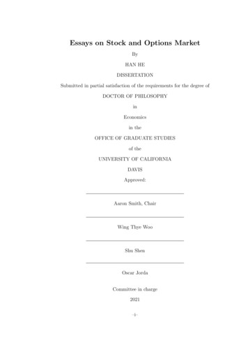
The table shows a comparison between three standard trading strategies. The trading results are computed by using the "SSE Composite Index." Strategy 1: using 100% available cash in daily trading, strategy 2: using 80% available cash in daily trading, strategy 3: using 50% available cash in daily trading.