Transcription
Partisan Spatial Sorting in the United States:A Theoretical and Empirical Overview Ethan Kaplan, University of MarylandJörg L. Spenkuch, Northwestern UniversityRebecca Sullivan, University of MarylandMarch 2022AbstractWe develop a variance-like index of heterogeneity in partisanship and use it to measure spatial sorting. We prove that our index is the only one (up to a linear transformation) that satisfies seven theoretical properties, all of which are intuitivelydesirable. Based on this index we document the long-run evolution of geographicsorting along partisan lines in the American electorate. We provide evidence thatspatial cleavages have increased dramatically since the mid-twentieth century. Atno point since the Civil War have partisans been as clustered within the boundariesof individual states as today. Nonetheless, even when geographic sorting is measured at the precinct level, differences across communities tend to be significantlysmaller than differences within. In this sense, the American electorate continues tobe more diverse within than across areas. We thank Jorge Perilla-Garcia and Daniel Kolliner for excellent research assistance. We have also benefited from helpful comments by Morris Fiorina, Jim Gimpel, Marc Hetherington, Greg Martin, Pablo Montagnes, Cody Tuttle, Haishan Yuan, and audience members at the 2018 APSA Annual Meeting. Any mistakes, however, are solely our own. Correspondence should addressed to edkaplan@umd.edu [Kaplan], orj-spenkuch@kellogg.northwestern.edu. [Spenkuch].
1. IntroductionAccording to popular perception, ordinary Americans are not only divided in their allegianceto one of the two major parties, but partisan divisions also manifest themselves across space.Republican supporters live in “red,” rural states, while Democrats reside in “blue,” urbanareas along the coasts. Some even argue that partisans have become so clustered in likeminded communities that the resulting spatial fissures are tearing American society apart(see, e.g., Bishop 2008). But how sorted are Americans really? And has the degree of sortingchanged much over time?In order to measure sorting and thereby answer these questions, we introduce a variance-likeindex of heterogeneity in ideology or partisanship. We show that our index is the only one thatsatisfies a set of seven intuitively desirable criteria. Chiefly among them, the variance indexallows us to exactly decompose overall heterogeneity in partisanship into differences acrossand within communities. As a result, we can gauge the degree of sorting along ideological linesby comparing partisan heterogeneity across areas to the heterogeneity within the respectivecommunities.Although we are primarily interested in partisan sorting, the usefulness of our index isnot limited to this particular context. Other applications might include (1) measuring thedegree of sorting by race across and within schools or classrooms, (2) comparing the degreeof educational sorting across and within firms, or (3) measuring the degree of sorting bycomparing heterogeneity in income at various levels of aggregation.After analytically developing our index, we use it to measure partisan geographic sortingdating back to 1856—the first presidential election with both a Democratic and a Republican candidate. Such a long horizon is useful for putting recent trends into perspective. Wecompare our measure of sorting to other common measures, most of which display overallsimilar trends. Our measure, however, has the advantage of being decomposable into constituent parts. This is important for comparing the degree of sorting across different levelsof aggregation, such as states, counties, and precincts.Our paper contributes both to the theory and to the empirical measurement of sorting.Although our analysis speaks to divisions within the American electorate by documentingtrends in partisan sorting over long periods of time, we do not directly contribute to thedebate on the causes and consequences of sorting (see, e.g., Bishop 2008; McDonald 2011;Gimpel and Hui 2015; Mummolo and Nall 2017; Martin and Webster 2018). We merely assessthe claim that partisans are increasingly clustered across space. To date, the literature hasfocused on potential downstream effects of sorting. Much less work has been done to directlyassess whether partisans are, in fact, more geographically sorted than in the past. Moreover,the little evidence that does exist is, for the most part, based on state-level differences,1
without a principled way of drawing comparisons over time (e.g., Glaeser and Ward 2006,Hopkins 2017). Glaeser and Ward’s (2006) assertion that partisan segregation is one of thebig myths of American electoral geography is, therefore, speculative.Two recent studies based on detailed voter-registration records do present evidence ofpartisan clustering. Brown and Enos (2021) use a snapshot from 2017 to show that, today,Democrats and Republicans are nearly as segregated as racial minorities. Sussell (2013)relies on data from California spanning the period from 1992 to 2010. His results suggestthat partisan segregation increased noticeably during this time.1Our analysis unearths a rich set of previously unknown facts. Specifically, we find that,within states, partisan sorting has increased approximately five fold between its nadir in 1976and the most recent presidential election in 2016. Surprisingly, since the 1970s, our measureof within-state geographic sorting is nearly perfectly correlated with Poole and Rosenthal’s(1997) well-known index of polarization in the U.S. House (ρ .95). Regardless of whetherwe measure within-state sorting at the county or precinct level, the data reveal a dramaticincrease in spatial differences—especially over the last five election cycles. Geographic sortingwithin states is currently at a historic high.2 Although we do find a rise in sorting acrossstates, the red-blue state divide is significantly lower than it was in the period surroundingthe Civil War or even in the mid-1890s through the mid-1920s. Moreover, the rise in statelevel partisan sorting is not nearly as sharp as the increase in sorting across counties withthe same state.Finally, though we document a dramatic rise in spatial sorting over the last few decades, allof our results imply that differences between individuals within counties or precincts are, onaverage, many times greater than differences across space. At the same time, we emphasizethat it is difficult to say how much geographic sorting is “too much.” Current levels are highby historical standards, and there simply does not exist enough evidence on the causal effectsof geographic cleavages on democratic outcomes to speculate about potential consequences.By developing a theoretically grounded measure of geographic sorting and by documenting1Specifically, Sussell (2013) computes isolation and segregation indices using partisan registration rates aswell as presidential election returns. Eleven of his twelve measures of partisan segregation increased duringthis period, with rates of growth ranging from 2.1% to 23.1%. (Brown and Enos 2021) compute isolationand exposure indices but only at one point in time.2In independent, simultaneous work, Darmofal and Strickler (forthcoming) also present time-series evidence on long-run sorting. An important difference between their approach and ours is that they rely onBishop’s (2008) concept of “landslide counties” to measure geographic sorting. As previously pointed outby Abrams and Fiorina (2012) and Klinkner (2004a; 2004b), using landslide counties to assess changes insorting is theoretically problematic because the results can be highly dependent on arbitrary cutoffs. As aconsequence, some of Darmofal and Strickler’s substantive conclusions differ greatly from ours. While theyfind that “the percentage of the voting public living in heavily or landslide partisan counties in the twentyfirst century is well within a normal historical range” (p. 83), we show that, when properly measured, currentlevels of voter partisan sorting are very high by historical standards.2
the recent increase therein, our analysis paves the way for research on a number of important questions related to political sorting. For instance, are spatial divisions in the electorallandscape a cause or a consequence of elite polarization? Does the clustering of like-mindedpartisans lead to better or worse representation? Does it cause legislative dysfunction? Doespartisan sorting create ideological echo chambers—as asserted by Bishop (2008)—or is itirrelevant for the evolution of voters’ views and preferences? On theoretical grounds theanswers to these questions are inherently ambigous. What our analysis establishes is that,today, partisans are more geographically clustered than at any time in recent memory.2. Measuring Geographic Sorting: TheoryBefore discussing our findings on historical patterns of geographical sorting by partisanship,we first ask how sorting on ideology should be measured in the first place. The literature hasheretofore been eclectic in its measurement of political sorting. Bishop (2008), for instance,calculates the share of voters living in “landslide counties,” i.e., counties in which one partyachieved a victory margin of at least 20%. Abrams and Fiorina (2012) criticize this measurefor being arbitrary and vague, and Klinkner (2004a; 2004b) shows that small definitionalchanges lead to as much as a 25% reduction in the number of voters in such counties.In what follows, we propose seven properties that any good measure of ideological heterogeneity ought to possess. The first six of them are self-evidently desirable, while the lastproperty is tailored towards comparing heterogeneity across and within regions. Being able tocompare heterogeneity across and within geographic areas is important because if partisanssort across space, then we would expect much of the extant heterogeneity to be captured bydifferences across rather than within communities.We prove that there exists one and only one (up to a constant positive multiple) indexthat satisfies all of our theoretical desiderata. To be clear, there is a vast literature that axiomatically derives different indices.3 Our contribution is to recognize that the mathematicalstructure of quantifying the degree of heterogeneity in ideology or partisanship is very similar to that of measuring inequality. We can, therefore, build upon prior work, particularlyBosman and Cowell (2010), and bring some of its insights to bear on our question. In ourdiscussion below, we motivate our axioms with reference to the measurement of partisansorting; however, as we have noted, there are many other potential applications. 4Mathematical Preliminaries.— We first assume that the researcher observes a valid proxy3See, e.g., Esteban and Ray (1994) for a well-known index of polarization.Our index is particularly useful when attempting to quantify nested sorting. Some examples besides theone presented in this paper would include sorting by race into school districts, into schools within districtsand into classrooms within schools; or sorting of workers by education level across industries, across firmswithin industries and across plants within firms.43
for voters’ ideology or partisanship.5 Formally, let there be n individuals, whose preferencesPare characterized by x (x1 , ., xn ). We use x̄ (1/n) ni 1 xi to denote the mean of x,while x̄ is an n 1 vector with x̄ in every position.Definition: An index of ideological heterogeneity is a function P that assigns a realnumber to any vector of preferences x, i.e., P : Rn R.Desirable Properties.— Any measure of ideological heterogeneity ought to have a well-definedand easily interpretable baseline. Our first axiom, therefore, states that measured heterogeneity should be equal to zero when all voters have identical preferences.Axiom 1 (normalization):P (x) 0 whenever xi xj for all i, j.In addition, an index of heterogeneity in ideology or partisanship should not change if votersbecome uniformly more liberal or conservative. As commonly understood, heterogeneityrefers to a divergence of preferences rather than the extremity of their mean. Hence, Axiom2 requires that uniform changes in voters’ preferences have no effect on P .Axiom 2 (translational invariance):P (x c) P (x) for any c (c, ., c) Rn .Since we are concerned with voters rather than political elites, we also think it desirablethat all individuals receive equal weight. That is, conditional on the distribution of preferences, measured heterogeneity should not depend on who holds which views (Axiom 3).Axiom 3 (anonymity):P (y) P (x) whenever y is simply a permutation of x.Nor should it matter how many individuals there are (Axiom 4). In particular, an exactdoubling of the population maintaining the distribution of preferences should not impact theindex.Axiom 4 (population independence):P (x, x) P (x).Independence of population size is important for directly comparing differently-sized groupsof voters. By imposing Axiom 4, we ensure that our conclusions about the evolution ofpartisan sorting across space and time are solely due to changes in the distribution of voters’preferences rather than differences in population size.Our next axiom requires that small changes in preferences lead only to small changes inmeasured heterogeneity.5In our empirical application, we use electoral returns to proxy for the partisanship of voters.4
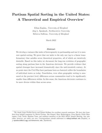
Axiom 5 (continuity):P is continuous in every element of x.Continuity fails for all indices that rely on cutoff values to classify states, counties, or anyother group of voters. Threshold-based indices are problematic because substantively minordifferences between voters across space or time may give the (false) impression of largedifferences or changes. Ansolabehere et al. (2006), for instance, argue that categorizing statesas either “red” or “blue” obscures the fact that most of America is actually “purple.” Klinkner(2004a; 2004b) makes a similar point when he criticizes Bishop’s (2008) measure of “landslidecounties.” He even demonstrates that small changes to the cutoff used to define “landslides”have a big effect on the results. By contrast, a continuous measure of voter heterogeneity isimmune to such problems.An important additional requirement is that as voters’ preferences diverge, measured heterogeneity increases.Axiom 6 (spread responsiveness):′some c 0, then P (x ) P (x).′If x (x1 , x2 ) with x1 x2 and x (x1 c, x2 c) forIn words, Axiom 6 deals with the minimal case of an electorate of only two individuals. If theideological distance between the two increases (without changing the mean), then measuredheterogeneity must go up. As an example, if there are no political differences among people,then our index should be zero; as differences emerge, our measure of heterogeneity should rise.Any index that does not satisfy this property is an inherently flawed measure of heterogeneityacross voters.6In our view, Axioms 1–6 are not controversial. They are desirable for any measure of voterheterogeneity. Our last axiom is the least trivial one. Yet, it is crucial for assessing theimportance of geographic divisions.As illustrated in Figure 1, even absent any macro-level differences in the overall compositionof the electorate, voters today might be living in more homogeneous communities than just afew decades ago. That is, they might be better sorted. Conversely, the American electorate asa whole might have become more polarized without any widening of spatial cleavages. Hence,assessing claims of spatial sorting involves a comparison of differences across and withincommunities. Put differently, we need to be able to disentangle communities becoming moreor less alike from changes in how internally differentiated the respective groups of voters are.6We define Axiom 6 in terms of two voters so that it is straightforward to say whether heterogeneity shouldbe increasing or decreasing. With three or more individuals, it is possible for an increased spread betweenone pair of individuals to coincide with a decline between other pairs, in which case it is a priori unclearwhether heterogeneity should go up or down.5
Figure 1: Heterogeneity Across vs. Within CommunitiesState 1State 2geographicallysortedgeographicallyhomogeneousTown ATown BIn addition, absent a commonly accepted definition of “community,” we need to be ableto consistently do so at different levels of spatial aggregation. Suppose, for instance, that,according to P , voters within every single electoral precinct in some state have become moreextreme over time, without any narrowing in the differences across precincts. Then if we useto P to asses heterogeneity in the state as a whole, it should also indicate rising heterogeneityat the state level. Axiom 7 ensures that this is the case.Axiom 7 (decomposability): There exists a nonnegative weighting function ω such that(i) P (x, y) ω(x̄, ȳ, nx , ny )P (x) ω(ȳ, x̄, ny , nx )P (y) P (x̄, ȳ) for all x Rnx and y Rny ;and (ii) ω(x̄, ȳ, nx , ny ) ω(ȳ, x̄, ny , nx ) 1.Intuitively, the axiom stipulates that a useful measure of heterogeneity ought to be decomposable into across- and within-group components.7 In our application, the former measuresgeographic sorting, i.e., the extent of mean differences across, say, states, counties, towns, orneighborhoods, etc. The latter is a weighted average of the heterogeneity within each groupof voters.Axiom 7 guarantees that these decompositions are exact and, when carried out at differentlevels of aggregation, mutually consistent. After all, it should be irrelevant whether we firstdecompose national differences to the state level and then to the county and precinct level,or if we directly work with the latter. In the remainder of this paper, we rely heavily on7We also note that we could alternatively look at voter heterogeneity across and between non-spatiallydefined groups. For example, we could use our index to look at heterogeneity within and across income oreducational groups at different levels of aggregation.6
decompositions at various levels of aggregation in order to assess whether Democratic andRepublican supporters are more geographically clustered today than in decades past. It is,therefore, important for P to ensure that our findings for different levels of aggregation aremutually consistent. Moreover, decomposability allows us to determine the relative importance of changes in sorting at different levels of aggregation, such as states, counties, orprecincts,As a technical matter, we restrict ω to be an arbitrary function of mean preferences aswell as groups’ sizes. We further require that all weights be non-negative and sum up to one.This last condition ensures that, if there are no mean differences across communities, thensociety as a whole shall not be deemed more (less) polarized than its most (least) polarizedsubgroup.A Unique Index.— We view each of the properties in Axioms 1–7 as desirable for an indexthat is being used to document geographic divisions over time. Given these axioms, we canformally prove that there exists a uniquely good measure.Proposition 1: An index satisfies Axioms 1–7 if and only if it is a positive scalar multiplePof P (x) (1/n) ni 1 (xi x̄)². Since P corresponds to the population variance, we refer tothis index as the variance index.In words, the proposition establishes that the variance index is the only measure of voterheterogeneity that has all of the desired properties. Any other index violates at least one ofour desiderata.8As a corollary to Proposition 1, the weights needed to disaggregate the variance indexacross different groups of voters are simply the groups’ population shares.Corollary:Suppose that P (x) satisfies Axioms 1–7, then ω(x̄ , ȳ, nx , ny ) nx.nx nyWhile Proposition 1 holds given any unidimensional representation of individuals’ preferences or actions, it is silent on how to best gauge ideology or partisanship. As a result,comparisons between different groups of voters may well depend on the underlying measureof preferences. We, therefore, advocate that the variance index be used with the understanding that any conclusion is inextricably tied to the representation of preference on which it isbased. That is, the variance index measures sorting in whatever facet of voters’ preferencesor actions is captured by x.8See Massey and Denton (1988) for a useful discussion of the properties of different measures of segregation,many of which may seem prima facie useful for measuring geographical sorting.7
3. Methods and Data3.1. Mapping Theory into DataSince we are interested in assessing the extent of spatial cleavages over long periods of time,most of our empirical application focuses on geographical sorting in partisanship as capturedby election results. Survey data would provide an alternative measure of partisan sentimentfrom which we could potentially compute partisan sorting. Unfortunately, survey data arescant before 1930 and rarely allow for systemic valid inferences below the state level eventoday. If we want to contrast geographic sorting today with the divisions that existed duringthe New Deal or during Reconstruction, we are forced to rely on electoral returns as a proxyfor voters’ partisan preferences.9To operationalize the theoretical insights in the previous section, consider a presidentialelection in which the Democratic candidate received nD votes, while the Republican onegarnered nR . We represent the choices of voters in this election by letting x be a vector withnD ones and nR zeros. Denoting the Democratic two-party vote share as v, the varianceindex simplifies to(1)P (x) 1 Dn (1 v)2 nR v 2 v(1 v),nwhere n nD nR . Based on this expression, P is minimized when all voters back thesame candidate, i.e., v 1 or v 0 and P (x) 0; it is maximized when the electorate isequally split, i.e., when v .5 so that P (x) .25.10 When interpreting the magnitude of thevariance index and its components, it is often useful to do so with these numbers in mind.In this context, it is important to distinguish ideological extremity from spatial sortingalong partisan lines. An area with a very high or very low Democratic vote share is likely anideologically extreme one. For instance, in 2016 three counties had a Democratic two-partyvote share below 5%: King County (TX), Roberts County (TX) and Garfield County (MT);while another sixty counties saw Democratic vote shares below 10%. On the Democratic side,in addition to the eight wards of Washington D.C., four counties had two-party Democraticvote share in excess of 90%: Prince George’s County (MD), Oglala Lakota County (SD),Bronx County (NY), and San Francisco County (CA). The aforementioned places are likelysome of the most partisan within the United States. They contribute substantially to partisan9We note that, in general elections in the U.S., there is rarely reason to cast strategic ballots. It is, therefore,reasonable to assume that votes proxy for partisan preferences.10We ignore votes for third-party candidates. The number of votes for these candidates is small in most,though not all, elections that we study. One advantage of our approach is that it easily accommodates thirdparty candidates as long as we have a good measure of the “partisan distance” between the independentcandidate and each of the other parties or candidates in the election.8
sorting across counties; internally, however, they are very homogeneous.By contrast, the Democratic and Republican two-party vote shares fell within 0.2 percentage points of parity in eight counties: Clark County (WA), Lorain County (OH), WinnebagoCounty (IL), Kent County (RI), Panola County (MS), Kendall County (IL), Nash County(NC), and Teton County (ID). These counties contributed the least to our measure of partisan sorting precisely because they had the greatest extent of internal heterogeneity.As matter of notation, when we measure differences across states, we let x̄s be an ns 1vector with the Democratic vote share in state s while, for each state, xs is an ns 1 vectorRwith nDs ones and ns zeros, one for each individual within the states. We then calculate theextent of sorting across states asSS(2)P (x̄1 , ., x̄s , ., x̄S ) {z} heterogeneity across states P (x) {z }overall heterogeneityX nsP (xs )n s 1 {z X nss 1n(vs v)2 .}heterogeneity within statesIn some of what follows, we report across-state sorting relative to the overall level ofpartisan heterogeneity, i.e., P (x̄1 , ., x̄s , ., x̄S )/P (x). We refer to this ratio as the acrossstate share and interpret it as the fraction of heterogeneity in partisanship that is attributableto systematic differences across states.To assess the relative importance of geographic cleavages at different levels of aggregation,we repeatedly applying our decomposition to geographic units that are nested. For instance,since counties are nested within states, we can further decompose equation (2) into(3)SP (x) {z }overall heterogeneity P (x̄1 , ., x̄s , ., x̄S ) {z}heterogeneity across statesSX ns s 1nP (x̄1,s , ., x̄c,s , ., x̄Cs ,s ) {z}within state heterogeneity across countiesCsXXnc,s s 1c 1n{zP (xc,s ) ,where Cs denotes the number of counties in state s, and xc,s represents the preference profileof voters in county c in the same state. Intuitively, the first term on the right-hand side inequation (3) measures the importance of differences in voters’ mean preferences across states.The second term tells us how geographically divided voters are, on average, across countieswithin the same state. The last term measures the degree of partisan heterogeneity withinindividual counties. Thus, our decomposition can be thought of as disentangling differencesbetween individuals within the same county from differences in the average across countieswithin the same state, as well as mean differences across states. Below, we demonstratethat the importance of these components varies considerably over the long arc of American9}heterogeneity within counties
history.For the most recent period, we also assess partisan sorting at the precinct level. Precinctlevel data allow us to document trends in geographic differences at a much finer scale, but onlyfor a shorter time frame and subject to the caveat that precinct boundaries are not temporallystable. Calculating precinct- rather than county-level heterogeneity in partisanship requiresnothing more than an appropriate change of indices in the equation above.113.2. Data SourcesWe obtained county-level presidential election returns for the years 1972 through 2016 fromthe CQ Voting and Elections Collection and the remainder from ICPSR (1999). Our countylevel time series starts in 1856, the first year in which both Democratic and Republicancandidates competed in a presidential election. Precinct-level electoral returns come primarily from the Harvard Election Data Archive. We collect electoral returns both for presidentialelections as well as elections for the House of Representatives. The precinct-level presidential election data is available from 2000 to 2016 whereas the precinct-level data on houseelections ends in 2012. Unfortunately, coverage of the Harvard Election Data Archive variessignificantly over time. Thus, whenever possible, we supplement the precint-level data withinformation form David Leip’s Atlas of U.S. Elections and with information that we collected directly from different Secretaries of State. The latter are additionally used to correcta number of anomalies in the raw data (see Appendix B for details).4. Partisan Sorting over Time: Evidence4.1. National Time SeriesWe now present our first decomposition of the variance index. We begin by calculating thedegree of partisan sorting across states because it is the highest interesting level of spatialaggregation and because “red states” and “blue states” have received substantial attentionin both the academic and popular discourse.Relying on the expression in equation (3), Figure 2 computes the total variance in twoparty votes for president and its decomposition into (1) an across-state component (shaded inblue), (2) a within-state across-county component (shaded in gray), and (3) a within-countycomponent (shaded in black). We present this decomposition for every presidential election11Note, our main results would remain qualitatively unchanged if we scaled votes in general elections by therespective candidates’ idealpoints. This is because for any two-candidate election, scaling votes correspondsto a linear transformation of x, which simply yields a scalar multiple of the variance index. In races withthree or more candidates, this equivalence need not hold. Candidates’ relative positions may affect bothlevels and shares of geographic heterogeneity among voters.10
Figure 2: Decomposition of the Variance Index, Presidential Elections 1856–2016Across-State ComponentWithin-State Across-County ComponentWithin-County Component.3Variance 02016YearNotes: Figure shows a decomposition of the variance index for each presidential election from 1856 to 2016. Asexplained in the text, the decomposition is based on the expression in equation (3).from 1856 through 2016.12 The blue area then corresponds to the first term on the right sideof equation (3), the gray area to the second term, and the black area to the third term.Figure 3 complements the previous figure by presenting the across-state and within-stateacross-county components as a fraction of the total variance index for the respective election. Doing so highlights the time trends in both measures of sorting. It also makes it morestraightforward to interpret their magnitudes and thus the change of relative partisan cleavages acros
big myths of American electoral geography is, therefore, speculative. Two recent studies based on detailed voter-registration records do present evidence of partisan clustering. Brown and Enos (2021) use a snapshot from 2017 to show that, today, Democrats and Republicans are nearly as segregated as racial minorities. Sussell (2013)