WIXLIB

Contents1 The challenge of fluid mechanics is mainly the kinematics of fluid flow.1.1Physical properties of materials; what distinguishes fluids from solids?1.1.11.1.25. . . . . . . . . . . .6The response to pressure — in linear deformation liquids are not very different fromsolids . . . . . . . . . . . . . . . . . . . . . . . . . . . . . . . . . . . . . . . . . . .8The response to shear stress — solids deform and fluids flow. . . . . . . . . . . . .101.2A first look at the kinematics of fluid flow . . . . . . . . . . . . . . . . . . . . . . . . . . . .141.3Two ways to observe fluid flow and the Fundamental Principle of Kinematics . . . . . . . . .151.4The goal and the plan of this essay; Lagrangian to Eulerian and back again . . . . . . . . . . .182 The Lagrangian (or material) coordinate system.202.1The joy of Lagrangian measurement . . . . . . . . . . . . . . . . . . . . . . . . . . . . . . .222.2Transforming a Lagrangian velocity into an Eulerian velocity . . . . . . . . . . . . . . . . . .232.3The Lagrangian equations of motion in one dimension . . . . . . . . . . . . . . . . . . . . .252.3.1Mass conservation; mass is neither lost or created by fluid flow . . . . . . . . . . . . .252.3.2Momentum conservation; F Ma in a one dimensional fluid flow . . . . . . . . . . .292.3.3The one-dimensional Lagrangian equations reduce to an exact wave equation . . . . .31The agony of the three-dimensional Lagrangian equations . . . . . . . . . . . . . . . . . . . .312.43 The Eulerian (or field) coordinate system.343.1Transforming an Eulerian velocity field to Lagrangian trajectories . . . . . . . . . . . . . . .353.2Transforming time derivatives from Lagrangian to Eulerian systems; the material derivative . .363.3Transforming integrals and their time derivatives; the Reynolds Transport Theorem . . . . . .383.4The Eulerian equations of motion . . . . . . . . . . . . . . . . . . . . . . . . . . . . . . . . .423.4.1Mass conservation represented in field coordinates . . . . . . . . . . . . . . . . . . .423.4.2The flux form of the Eulerian equations; the effect of fluid flow on properties at a fixedposition . . . . . . . . . . . . . . . . . . . . . . . . . . . . . . . . . . . . . . . . . .453.4.3Momentum conservation represented in field coordinates . . . . . . . . . . . . . . . .463.4.4Fluid mechanics requires a stress tensor (which is not as difficult as it first seems) . . .483.4.5Energy conservation; the First Law of Thermodynamics applied to a fluid . . . . . . .54A few remarks on the Eulerian equations . . . . . . . . . . . . . . . . . . . . . . . . . . . . .553.54 Depictions of fluid flows represented in field coordinates.564.1Trajectories (or pathlines) are important Lagrangian properties . . . . . . . . . . . . . . . . .564.2Streaklines are a snapshot of parcels having a common origin . . . . . . . . . . . . . . . . . .574.3Streamlines are parallel to an instantaneous flow field . . . . . . . . . . . . . . . . . . . . . .595 Eulerian to Lagrangian transformation by approximate methods.461

1 THE CHALLENGE OF FLUID MECHANICS IS MAINLY THE KINEMATICS OF FLUID FLOW.5.15.25Tracking parcels around a steady vortex given limited Eulerian data . . . . . . . . . . . . . .615.1.1The zeroth order approximation, or PVD . . . . . . . . . . . . . . . . . . . . . . . .615.1.2A first order approximation, and the velocity gradient tensor . . . . . . . . . . . . . .63Tracking parcels in gravity waves . . . . . . . . . . . . . . . . . . . . . . . . . . . . . . . .645.2.1The zeroth order approximation, closed loops . . . . . . . . . . . . . . . . . . . . . .655.2.2The first order approximation yields the wave momentum and Stokes drift . . . . . . .656 Aspects of advection, the Eulerian representation of fluid flow.686.1The modes of a two-dimensional thermal advection equation . . . . . . . . . . . . . . . . . .696.2The method of characteristics implements parcel tracking as a solution method . . . . . . . .716.3A systematic look at deformation due to advection; the Cauchy-Stokes Theorem . . . . . . . .756.3.1The rotation rate tensor . . . . . . . . . . . . . . . . . . . . . . . . . . . . . . . . . .786.3.2The deformation rate tensor . . . . . . . . . . . . . . . . . . . . . . . . . . . . . . .806.3.3The Cauchy-Stokes Theorem collects it all together . . . . . . . . . . . . . . . . . . .827 Lagrangian observation and diagnosis of an oceanic flow.848 Concluding remarks; where next?879 Appendix: A Review of Composite Functions8819.1Definition . . . . . . . . . . . . . . . . . . . . . . . . . . . . . . . . . . . . . . . . . . . . .899.2Rules for differentiation and change of variables in integrals . . . . . . . . . . . . . . . . . .90The challenge of fluid mechanics is mainly the kinematics of fluid flow.This essay introduces a few of the concepts and mathematical tools that make up the foundation of fluidmechanics. Fluid mechanics is a vast subject, encompassing widely diverse materials and phenomena. Thisessay emphasizes aspects of fluid mechanics that are relevant to the flow of what one might term ordinaryfluids, air and water, that make up the Earth’s fluid environment. 1;2 The physics that govern the geophysicalflow of these fluids is codified by the conservation laws of classical mechanics: conservation of mass, andconservation of (linear) momentum, angular momentum and energy. The theme of this essay follows from thequestion — How can we apply these conservation laws to the analysis of a fluid flow?In principle the answer is straightforward; first we erect a coordinate system that is suitable fordescribing a fluid flow, and then we derive the mathematical form of the conservation laws that correspond to1 Footnotesprovide references, extensions or qualifications of material discussed in the main text, along with a few homeworkassignments. They may be skipped on first reading.2 An excellent web page that surveys the wide range of fluid mechanics is http://physics.about.com/cs/fluiddynamics/

1 THE CHALLENGE OF FLUID MECHANICS IS MAINLY THE KINEMATICS OF FLUID FLOW.6that system. The definition of a coordinate system is a matter of choice, and the issues to be considered aremore in the realm of kinematics — the description of fluid flow and its consequences — than of dynamics orphysical properties. However, the physical properties of a fluid have everything to do with the response to agiven force, and so to appreciate how or why a fluid is different from a solid, the most relevant physicalproperties of fluids and solids are reviewed briefly in Section 1.1.Kinematics of fluid flow are considered beginning in Section 1.2. As we will see in a table-topexperiment, even the smallest and simplest fluid flow is likely to be fully three-dimensional andtime-dependent. It is this complex kinematics, more than the physics per se, that makes classical andgeophysical fluid mechanics challenging. This kinematics also leads to the first requirement for a coordinatesystem, that it be able to represent the motion and properties of a fluid at every point in a domain, as if thefluid material was a smoothly varying continuum. Then comes a choice, discussed beginning in Section 1.3and throughout this essay, whether to observe and model the motion of moving fluid parcels, the Lagrangianapproach that is closest in spirit to solid particle dynamics, or to model the fluid velocity as observed fixedpoints in space, the Eulerian approach. These each have characteristic advantages and both are systems arewidely used, often side-by-side. The transformation of conservation laws and of data from one system to theother is thus a very important part of many investigations and is the object at several stages of this essay.1.1 Physical properties of materials; what distinguishes fluids from solids?Classical fluid mechanics, like classical thermodynamics, is concerned with macroscopic phenomena (bulkproperties) rather than microscopic (molecular-scale) phenomena. In fact, the molecular makeup of a fluidwill be studiously ignored in all that follows, and the crucially important physical properties of a fluid, e.g., itsmass density, , heat capacity, Cp, among others, must be provided from outside of this theory, Table (1). Itwill be assumed that these physical properties, along with flow properties, e.g., the pressure, P , velocity, V ,temperature, T , etc., are in principle definable at every point in space, as if the fluid was a smoothly varyingcontinuum, rather than a swarm of very fine, discrete particles (molecules). 3The space occupied by the material will be called the domain. Solids are materials that have a more orless intrinsic configuration or shape and do not conform to their domain under nominal conditions. Fluids donot have an intrinsic shape; gases are fluids that will completely fill their domain (or container) and liquids arefluids that form a free surface in the presence of gravity.An important property of any material is its response to an applied force, Fig. (1). If the force on the faceof a cube, say, is proportional to the area of the face, as will often be the case, then it is appropriate toconsider the force per unit area, called the stress, and represented by the symbol S ; S is a three componentstress vector and S is a nine component stress tensor that we will introduce briefly here and in much moredetail in Section 3.4. The SI units of stress are Newtons per meter squared, which is commonly representedby a derived unit, the Pascal, or Pa. Why there is a stress and how the stress is related to the physicalproperties and the motion of the material are questions of first importance that we will begin to consider inthis section. To start we can take the stress as given.3 Readersare presumed to have a college-level background in physics and multivariable calculus and to be familiar with basicphysical concepts such as pressure and velocity, Newton’s laws of mechanics and the ideal gas laws. We will review the definitionswhen we require an especially sharp or distinct meaning.

1 THE CHALLENGE OF FLUID MECHANICS IS MAINLY THE KINEMATICS OF FLUID FLOW.7Some physical properties of air, sea and land (granite)airsea watergranitedensity , kg m 31.210252800heat capacityCp; J kg 1 C 1100040002800bulk modulusB, Pa1.3 1052.2 1094 1010sound speedc, m s 133015005950shear modulusK, Panana2 1010viscosity , Pa s18 10 61 10 3 1022Table 1: Approximate, nominal values of some thermodynamic variables that are required to characterizematerials to be described by a continuum theory. These important data must be derived from laboratorystudies. For air, the values are at standard temperature, 0 C, and nominal atmospheric pressure, 105 Pa. Thebulk modulus shown here is for adiabatic compression; under an isothermal compression the value for air isabout 30% smaller; the values are nearly identical for liquids and solids. na is not applicable. The viscosity ofgranite is temperature-dependent; granite is brittle at low temperatures, but appears to flow as a highly viscousmaterial at temperatures above a few hundred C.Figure 1: An orthogonal triad of Cartesian unit vectors and a small cube of material. The surroundingmaterial is presumed to exert a stress, S , upon theface of the cube that is normal to the z axis. Theoutward-directed unit normal of this face is n D ez .To manipulate the stress vector it will usually be necessary to resolve it into components: S zz is the projection of S onto the ez unit vector and is negative,and Sxz is the projection of S onto the ex unit vector and is positive. Thus the first subscript on S indicates the direction of the stress component and thesecond subscript indicates the orientation of the faceupon which it acts. This ordering of the subscriptsis a convention, and it is not uncommon to see thisreversed.

1 THE CHALLENGE OF FLUID MECHANICS IS MAINLY THE KINEMATICS OF FLUID FLOW.8The component of stress that is normal to the upper surface of the material in Fig. (1) is denoted Szz . Anormal stress can be either a compression, if Szz 0, as implied in Fig. (2), or a tension, if Szz 0. Themost important compressive normal stress is almost always due to pressure rather than to viscous effects, andwhen the discussion is limited to compressive normal stress only we will identify Szz with the pressure.1.1.1The response to pressure — in linear deformation liquids are not very different from solidsEvery material will undergo some volume change as the ambient pressure is increased or decreased, thoughthe amount varies quite widely from gases to liquids and solids. To make a quantitative measure of thevolume change, let P0 be the nominal pressure and h0 the initial thickness of the fluid sample; denote thepressure change by ıP and the resulting thickness change by ıh. The normalized change in thickness, ıh h0 ,is called the linear deformation (linear in this case meaning that the displacement is in line with the stress).The linear deformation is of special significance in this one-dimensional configuration because the volumechange is equal to the linear deformation, ıV D V0 ıh h0 (in a two- or three-dimensional fluid this need notbe the case, Section 6.3). The mass of material, M D V , is not affected by pressure changes and hence themass density, D M V , will change inversely with the linear deformation;ı D 0ıVDV0ıh;h0(1)where ı is a small change, ı 1. Assuming that the dependence of thickness change upon pressure can beobserved in the laboratory, then ıh D ıh.P0 ; ıP / together with Eq. (1) are the rudiments of an equation ofstate, the functional relationship between density, pressure and temperature, D .P; T / or equivalently,P D P . ; T /, with T the absolute temperature in Kelvin.The archetype of an equation of state is that of an ideal gas, P V D nRT where n is the number ofmoles of the gas and R D 8:31 Joule moles 1 K 1 is the universal gas constant. An equivalent form thatshows pressure and density explicitly isP D RT M;(2)where D nM V is the mass density and M is the molecular weight (kg/mole). If the composition of thematerial changes, then the appropriate equation of state will involve more than three variables, for examplethe concentration of salt if sea water, or water vapor if air.An important class of phenomenon may be described by a reduced equation of state having statevariables density and pressure alone, D .P /; or equivalently, P D P . /:(3)It can be presumed that is a monotonic function of P and hence that P . / should be a well-defined functionof the density. A fluid described by Eq. (3) is said to be ‘barotropic’ in that the gradient of density will beeverywhere parallel to the gradient of pressure, r D .@ @P /rP , and hence surfaces of constant densitywill be parallel to surfaces of constant pressure. The temperature of the fluid will change as pressure work isdone on or by the fluid, and yet temperature need not appear as a separate, independent state variableprovided conditions approximate one of two limiting cases: If the fluid is a fixed mass of ideal gas, say, thatcan readily exchange heat with a heat reservoir having a constant temperature, then the gas may remain

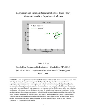
1 THE CHALLENGE OF FLUID MECHANICS IS MAINLY THE KINEMATICS OF FLUID FLOW.9Figure 2: A solid or fluid sample confined within a piston has a thickness h0 at the ambient pressure P0 . Ifthe pressure is increased by an amount ıP , the material will be compressed by the amount ıh and the volumedecreased in proportion. The work done during this compression will raise the temperature of the sample,perhaps quite a lot if the material is a gas, and we have to specify whether the sidewalls allow heat flux intothe surroundings (isothermal compression) or not (adiabatic compression); the B in Table 1 is the latter.isothermal under pressure changes and so D 0P 0; or, P D P0 :P0 (4)The other limit, which is more likely to be relevant, is that heat exchange with the surroundings is negligiblebecause the time scale for significant conduction is very long compared to the time scale (lifetime or period)of the phenomenon. In that event the system is said to be adiabatic and in the case of an ideal gas the densityand pressure are related by the well-known adiabatic law, 4 D 0 .P 1 / ; or, P D P0 . / :P0 0(5)The parameter D Cp Cv is the ratio of specific heat at constant pressure to the specific heat at constantvolume; 1:4 for air and nearly independent of pressure or density. In an adiabatic process, the gastemperature will increase with compression (work done on the gas) and hence the gas will appear to be lesscompressible, or stiffer, than in an otherwise similar isothermal process, Eq. (2).A convenient measure of the stiffness or inverse compressibility of the material isBDSzzDıh hV0ıPıPD 0 ;ıVı (6)called the bulk modulus. Notice that B has the units of stress or pressure, Pa, and is much like a normalizedspring constant; B times the normalized linear strain (or volume change or density change) gives the resultingpressure change. The numerical value of B is the pressure increase required to compress the volume by 100%of V0 . Of course, a complete compression of that sort does not happen outside of black holes, and the bulkmodulus should be regarded as the first derivative of the state equation, accurate for small changes around theambient pressure, P0 . Gases are readily compressed; a pressure increase ıP D 104 Pa, which is 10% above4 Anexcellent online source for many hysics;

1 THE CHALLENGE OF FLUID MECHANICS IS MAINLY THE KINEMATICS OF FLUID FLOW. 10nominal atmospheric pressure, will cause an air sample to compress by about B 1 104 P a D ıV Vo D 7%under adiabatic conditions. Most liquids are quite resistant to compressive stress, e.g., for water,B D 2:2 109 Pa, which is less than but comparable to the bulk modulus of a very stiff solid, granite (Table1). Thus the otherwise crushing pressure in the abyssal ocean, up to about 1000 times atmospheric pressure inthe deepest trench, has a rather small effect upon sea water, compressing it and raising the density by onlyabout five percent above sea level values. Water is stiff enough and pressure changes associated withgeophysical flows small enough that for many purposes water may be idealized as an incompressible fluid, asif B was infinite. Surprisingly, the same is often true for air.The first several physical properties listed in Table 1 suggest that water has more in common with granitethan with air, our other fluid. The character of fluids becomes evident in their response to anything besides acompressive normal stress. Fluids are qualitatively different from solids in their response to a tensile normalstress, i.e., Szz 0, is resisted by many solid materials, especially metals, with almost the same strength thatthey exhibit to compression. In contrast, gases do not resist tensile stress at all, while liquids do so only very,very weakly when compared with their resistance to compression. Thus if a fluid volume is compressed alongone dimension but is free to expand in a second, orthogonal, direction (which the one-dimensional fluidconfined in a pistion, Fig. (2), can not, of course) then the volume may remain nearly constant though thefluid may undergo significant linear deformation, compession and a compensating expansion, in orthogonaldirections.1.1.2The response to shear stress — solids deform and fluids flowA stress that is parallel to (in the plane of) the surface that receives the stress is called a ‘shear’ stress. 5 Ashear stress that is in the x direction and applied to the upward face of the cube in Fig. (1) would be labeledSxz and a shear stress in the y-direction, Syz . A measure of a material’s response to a steady shear stress is theshear deformation, r h, where r is the steady (equilibrium) sideways displacement of the face that receivesthe shear stress and h is the column thickness (Fig. 3, and note that the cube of material is presumed to bestuck to the lower surface). The corresponding stiffness for shear stress, or shear modulus, is then defined asKDSxz;r h(7)which has units of pressure. The magnitude of K is the shear stress required to achieve a shear deformation ofr h D 1, which is past the breaking point of most solid materials. For many solids the shear modulus iscomparable to the bulk modulus (Table 1). 6Fluids are qualitatively different from solids in their response to a shear stress. Ordinary fluids such asair and water have no intrinsic configuration, and hence fluids do not develop a restoring force that can5 Theword shear has an origin in the Middle English scheren, which means to cut with a pair of sliding blades (as in ‘Why are youscheren

theory (forward calculation) in fluid mechanics is developed within the Eulerian system. Lagrangian and Eulerian concepts and methods are thus used side-by-side in many investigations, and the premise of this essay is that an understanding of both systems and the relationships between them can help form the framework for a study of fluid .