Transcription
STATISTICAL PARAMETRIC MAPPING (SPM): THEORY, SOFTWARE AND FUTURE DIRECTIONS1Todd C Pataky, 2Jos Vanrenterghem and 3Mark Robinson1Shinshu University, Japan2Katholieke Universiteit Leuven, Belgium3Liverpool John Moores University, UKCorresponding author email: tpataky@shinshu-u.ac.DESCRIPTIONOverview— Statistical Parametric Mapping (SPM) [1] wasdeveloped in Neuroimaging in the mid 1990s [2], primarilyfor the analysis of 3D fMRI and PET images, and hasrecently appeared in Biomechanics for a variety ofapplications with dataset types ranging from kinematic andforce trajectories [3] to plantar pressure distributions [4](Fig.1) and cortical bone thickness fields [5].SPM’s fundamental observation unit is the “mDnD”continuum, where m and n are the dimensionalities of theobserved variable and spatiotemporal domain, respectively,making it ideally suited for a variety of biomechanicalapplications including: (m 1, n 1) Joint flexion trajectories (m 3, n 1) Three-component force trajectories (m 1, n 2) Contact pressure distributions (m 6, n 3) Bone strain tensor fields.SPM handles all data types in a single, consistent statisticalframework, generalizing to arbitrary data dimensionalitiesand geometries through Eulerian topology.Table 1: Many types of biomechanical data are mDnD, butmost statistical tests in the literature are 1D0D: t tests,regression and ANOVA, and based on the relatively simpleGaussian distribution, despite nearly a century of theoreticaldevelopment in mD0D and mDnD statistics.TheoryApplied1D dataScalarVector1D1DmD1DRandom FieldTheorySPMThe purposes of this workshop are:1.2.3.Although SPM may appear complex it is relatively easy toshow that SPM reduces to common softwareimplementations (SPSS, R, MATLAB, etc.) when m 1 andn 0. Identically, it is conceptually easy to show howcommon tests, ranging from t tests and regression toMANCOVA, all generalize to SPM when one’s data movefrom 0D scalars (1D0D) to mDnD continua (Table 1).0D dataVectormD0DMultivariateGaussianGaussianT testsT2 testsRegressionCCAANOVAMANOVAScalar1D0D4.5.To review SPM’s historical context.To demonstrate how SPM generalizes common tests(including t tests, regression and ANOVA) to thedomain of mDnD data.To clarify potential pitfalls associated with the use of0D approaches to analyze nD data.To provide an overview of spm1d (www.spm1d.org),open-source software (Python, MATLAB) for theanalysis of mD1D continua, and how it can be used toanalyze a variety of biomechanical datasets.To discuss future directions for SPM in Biomechanics.Target Audience— Scientists, clinicians and engineers whodeal with spatiotemporally continuous data, and allindividuals interested in alternatives to simple classicalhypothesis testing.Figure 1: SPM first made the jump from Neuroimaging (a)to Biomechanics (b) in 2008 in plantar pressure analysis [5]and has since emerged in a variety of biomechanicsapplications including: kinematics/ force trajectory analysisand finite element modeling. SPM using topologicalinference to identify continuum regions (depicted as warmcolors) that significantly co-vary with an experimentaldesign.Expected audience background— Experience analyzing kinematics / dynamics time series Basic familiarity with MATLAB Familiarity with t tests, regression and ANOVAAdditionally, advanced topics toward the end of theworkshop will be directed toward attendees who havefamiliarity with or who are interested in: Repeated measures modeling Multivariate statistics Bayesian modeling and analysisLearning Objectives—1) How and why SPM works: its fundamental concepts.2) How to access and use spm1d software to conductcommon analyses of 1D biomechanics data.3) How to interpret and report SPM results.
PROGRAMTime0:00 – 0:300:30 – 1:001:00 – 1:301:30 – 1:451:45 – ContentBackground & TheorySoftwareInterpretation & ReportingFuture DirectionsOpen Discussion(The last 5 minutes of each session will be devoted to Q&A)Background & Theory— First we promote critical thinkingregarding statistics by interactively reviewing the meaningof experimentation, random sampling and probabilityvalues. Through random simulations of 0D data and 1D datawe clarify that statistical tests, while used for experimentalanalyses, are more aptly summarized as descriptors ofrandomness. This will prepare attendees to make theapparent leap but actual small step into the world of SPM:by observing what 1D randomness looks like (Fig.2), andhow it can be funneled into t tests, just like the 0D Gaussian,it will become easy for attendees to conceptually connect thesimple t test to its nD SPM manifestations (Table 1). Just ast tests’ p values emerge directly from Gaussian theory,SPM’s p values emerge directly from RFT. Coupled withan explanation of SPM’s evolution in both Neuroimagingand Biomechanics, attendees will understand that SPMrepresents a natural progression of classical statisticsconcepts.Software— Procedural knowledge will be stressed through aMatlab demonstration of spm1d basics (www.spm1d.org),its relation to other software packages, and its broadercapabilities. Data organization and tests’ optionalparameters (e.g. one- vs. two-tailed, sphericity assumptions,etc.) will be described through example and with referenceto online documentation. Additionally, spm1d’s collectionof real and simulated datasets will be introduced andexplored. We’ll finally introduce spm1d’s online forums forfree software support and general statistics discussion.Interpretation & Reporting— We will next guide attendeesthrough experimental design, scientific interpretation andreporting of SPM results. Necessary details includingexperimental design parameters, SPM-specific parameters,will be emphasized. Key literature references will besummarized. For a practical demonstration we will revisitsome datasets from our own papers to discuss real Methodsand Results reporting. We emphasize these points throughhypothetical examples of bad SPM reporting. We finish bysummarizing literature and internet resources for continuedSPM learning.Future Directions— We will provide an update regardingspm1d’s current state, including a variety of functionalitywe have in the development pipeline including: normality,power analysis, and Bayesian inference. We will alsodiscuss spm1d’s possible expansion into the 2D and 3Ddomains, as a light-weight Biomechanics-friendly version ofgold-standard Neuroimaging software. We will also brieflyrevisit theory to summarize SPM’s relation to other wholedataset techniques from the Biomechanics literatureincluding: principal components analysis, wavelet analysisand functional data analysis. We will end with an openQ&A session regarding our spm1d software, SPMmethodology in general, and other aspect of the workshop.Figure 2: Depiction of Random Field Theory’s model of1D randomness. Fluctuations about means are modeled assmooth continua, parameterized by the FWHM (full-widthat half-maximum) of a Gaussian kernel which is convolvedwith pure 1D noise. As FWHM approaches , the dataapproach 0D, and SPM results approach those fromcommon software implementations. By seeing how both 0DGaussian data and these random can be routed into a t test,attendees will realize that t tests (and all other tests) simplyfunnel randomness into a test statistic, and thus the onlydifference between SPM and common 0D techniques is theform of randomness one assumes.LIST OF SPEAKERS(page 3)REFERENCES1. Friston KJ, et al. Statistical Parametric Mapping: TheAnalysis of Functional Brain Images, Elsevier, 2007.2. Friston KJ, et al. Human Brain Mapping. 2(4), 189-210,1995.3. Pataky TC, et al. Journal of Biomechanics 46(14):2394-2401, 2013.4. Pataky TC, et al. Journal of Biomechanics, 41(9),1987-1994, 2008.5. Li W, et al. Bone, 44(4), 596-602, 2009.
LIST OF SPEAKERSTodd C. Pataky, Ph.D., Associate ProfessorInstitute for Fiber Engineering, Shinshu UniversityDepartment of BioengineeringTokida 3-15-1, Ueda, Nagano, JAPAN 386-8567tpataky@shinshu-u.ac.jpTodd Pataky received a Ph.D. in Kinesiology and Mechanical Engineering from thePennsylvania State University in 2004 and pursued postdoctoral research positions infunctional neuroimaging and biomechanical continuum analysis in Japan (ATRInternational, Kyoto) and the UK (University of Liverpool). He is currently an AssociateProfessor in the Institute for Fiber Engineering, Shinshu University (Japan) where hisresearch focuses on the development of continuum statistics techniques and theirapplications in Biomechanics. He has over 60 peer-reviewed publications inBiomechanics, many of which focus on SPM and its applications. Notable honors include:Young Investigator Award (bronze) at the World Congress on Biomechanics (2010), NikeAward for Athletic Footwear Research (2009), and William Evans Fellow at theUniversity of Otago, New Zealand (2014).Mark Robinson, Ph.D., Senior LecturerResearch Institute for Sport and Exercise SciencesLiverpool John Moores UniversityTom Reilly Building, Byrom StreetLiverpool, UK L3 3AFM.A.Robinson@ljmu.ac.ukMark is currently a Senior Lecturer in Biomechanics and Programme Leader for theBSc(Hons) Sport and Exercise Sciences degree at LJMU. He completed his doctorate in2011 in the School of Sport and Exercise Sciences, LJMU. His research interests arerelated to musculoskeletal loading, injury and impairment in the lower limbs, specificallyduring dynamic sporting activities. Of particular interest are knee injuries, player loadingin soccer, and gait analysis. His research also includes the development of SPM as amethod to provide biomechanists with the appropriate statistical tools to analyze complexbiomechanical data. He has published over 30 journal articles in these areas since 2012 andwas awarded a UEFA Research Grant in 2014.Jos Vanrenterghem, Ph.D., Associate ProfessorKU Leuven, Department of Rehabilitation SciencesTervuursevest 101 - box 15013001 Leuven, Belgiumjos.vanrenterghem@kuleuven.beJos received a PhD in Biomechanics from Ghent University in 2004. After having lecturedat the School of Sport and Exercise Sciences at Liverpool John Moores University for 10years, he is now an Associate Professor at the University of Leuven. He has published over50 articles in peer-reviewed Biomechanics journals, with research interests in lowerextremity musculoskeletal loading mechanisms and injury prevention in sport. He has beenteaching biomechanics across undergraduate and postgraduate levels, providing him with agood insight in the common issues that students face when analyzing biomechanical data.He has also delivered a series of workshops on research practice in Biomechanics, anddevotes much of his work to making biomechanics available in applied and clinicalcontexts, including through the use of SPM.
STATISTICAL PARAMETRIC MAPPINGTHEORY, SOFTWARE AND FUTURE DIRECTIONSTodd PatakyJos VanrenterghemMark RobinsonDept. of BioengineeringDept. of RehabilitationSciencesInstitute for Sport andExercise Sciences26 July 2017ISB Brisbane
Overview 17:00 – 17:3017:30 – 18:0018:00 – 18:3018:30 – 18:4018:40 –26 July 2017ISB BrisbaneBackground & TheorySoftwareInterpretation & ReportingFuture DirectionsOpen Discussion
BACKGROUND & THEORYTodd Pataky26 July 2017ISB Brisbane
SSTATISTICALProbabilistic inferences regardingexperimental dataPPARAMETRIC- Based on mean & SD & sample size- Also non-parametric (SnPM)- Parameterized model of cerebral blood flowMMAPPINGResults form an n-Dimensional “map”in the same space as the original data(i.e. test statistics [t and F] are n-D continua)
n-D continuaSmooth, bounded
n-D, m-D continuacontinuumdependent variableUnivariate 0DBody mass0D, 1DMultivariate 0DGRF at t 50 ms0D, 3DUnivariate 1DKnee flexion1D, 1DMultivariate 1DKnee posture1D, 6DUnivariate nDFoot pressure2D, 1DMultivariate nDBone strain tensor3D, 6DSPSSMATLABR
A brief history of SPM1976 Adler & Hasofer, Annals of Prob.1990 Friston et al. J Cerebral Blood Flow1995 Friston et al. Human Brain Mapping8663 citationsH-index: 202i-10-index: 7582004 Worsley et al. NeuroImage2008 Pataky et al. New insights into the plantar pressure correlatesof walking speed using pedobarographic statistical parametric mappingJ Biomech 41: 1987-1994.2009 Li et al. Identify fracture-critical regions inside the proximalfemur using statistical parametric mapping, Bone 44: 596-602
Example
What is a p value?Demo
What is a p value?The probability that a randomprocess will yield a particularresult.
Infinite set of experimentsRandomdataExperimenttwo sampleMetrict valueOne experimentp value
t and F values describe one experimentp values describe the behavior of randomdata in an infinite set of experimentsUse nD random data to make probabilisticconclusions regarding nD experimental data
www.spm1d.org
spm1d.org/rft1dPataky (2016) J. Statistical Software
Statistics ztF𝛘2T2DistributionFunctions probability density survival function inverse survival function
ANNICASVMkPCASOM
www.spm1d.org
spm1d tutorial, ISB 2017Mark A. RobinsonLiverpool John Moores University, UKm.a.robinson@ljmu.ac.ukThis tutorial will focus on using the software and will cover:1.2.3.4.5.6.getting "spm1d"input data organisationstatistical tests: t-tests, regression, ANOVA, CCAkeywordshelpquestions?1. Software"spm1d" is an open source package for one-dimensional StatisticalParametric Mapping.The current version is 0.4The python code repository is: .com/0todd0000/spm1d/)The matlab code repository //github.com/0todd0000/spm1dmatlab)
2. Input data organisationUnivariate spm1d uses a (J x Q) array, where J is the number of 1Dresponses (i.e. trials or subjects) and Q is the number of nodes in the 1Dcontinuum.e.g. 10 subject means normalized to 101 nodes will give a10x101 arrayMultivariate spm1d analysis the data should be arranged as a (J x Q x I)array, where I is the number of vector components in the 1D continuum.e.g. 10 subject means normalized to 101 nodes for GRFX,Y,Z, will give a 10x101x3 vector field3. Statistical testsa. 1D two-sample t-test/examples/stats1d/ex1d ttest2.m
In [2]:% load some datadataset spm1d.data.uv1d.t2.PlantarArchAngle();[YA,YB] deal(dataset.YA, dataset.YB);datasetdataset struct with fields:cite: 'Caravaggi, P., Pataky, T., G?nther, M., Savage, R., & Crompton, R. (2010). Dynamics of longitudinal arch support in relation to walking speed: contribution of the plantar aponeurosis. Journal of Anatomy, 217(3), 254?261. : [10 101 double]YB: [10 101 double]This dataset has two variables both of size 10x101spm1d has built in plotting functions for data e.g. plot meanSD
In [3]:% Plot the dataspm1d.plot.plot meanSD(YA,'color','r');hold onspm1d.plot.plot meanSD(YB,'color','b');
In [4]:%(1) Conduct SPM analysis:spm spm1d.stats.ttest2(YA, YB);spmi spm.inference(0.05, 'two tailed',true);disp(spmi)SPM{t} inferencez: [1 101 double]df: [1 18]fwhm: 20.5956resels: [1 4.8554]alpha: 0.0500zstar: 3.2947p set: 0.0312p: 0.0312
In [5]:% Plot SPM analysis outcomespmi.plot();spmi.plot threshold label();spmi.plot p values();
In [6]:% For descriptive information about clustersspmi.clusters{1,1}ans Cluster with R:h:xy:P:[93.2746 100]106.72540.32653.2947[96.5343 4.5976]0.0312b. 1D Linear Regression/examples/stats1d/ex1d regression.m
In [7]:% Load example datadataset spm1d.data.uv1d.regress.SpeedGRF();[Y,x] deal(dataset.Y, dataset.x);datasetdataset struct with fields:cite: 'Pataky, T. C., Caravaggi, P., Savage, R.,Parker, D., Goulermas, J., Sellers, W., & Crompton,R. (2008). New insights into the plantar pressure correlates of walking speed using pedobarographic statistical parametric mapping (pSPM). Journal of Biomechanics, 41(9), 1987?1994.'Y: [60 101 double]x: [60 1 double]
In [8]:% Plot the GRF dataplot(Y');xlabel('Stance %');ylabel('Force (N/BW)');
In [9]:subplot(221);scatter(x,Y(:,20)); title('20%');bel('Force (N/BW)'); lsline()subplot(222);scatter(x,Y(:,50)); title('50%');bel('Force (N/BW)'); lsline()subplot(223);scatter(x,Y(:,92)); title('92%');bel('Force (N/BW)'); lsline()xlabel('speed (m/s)');ylaxlabel('speed (m/s)');ylaxlabel('speed (m/s)');yla
In [10]:% Conduct SPM analysis:spm spm1d.stats.regress(Y, x);spmi spm.inference(0.05, 'two tailed', true);disp(spmi)SPM{t} inferencez: [1 101 double]df: [1 58]fwhm: 6.1343resels: [1 16.3017]alpha: 0.0500zstar: 3.3945p set: 4.0634e-14p: [0 0 0 0.0017]
In [11]:% Plot SPM outputspmi.plot();spmi.plot threshold label();spmi.plot p values();c. ANOVA - between groups/examples/stats1d/ex1d anova1.mIn [12]:% Load data:dataset spm1d.data.uv1d.anova1.SpeedGRFcategorical();[Y,A] deal(dataset.Y, dataset.A);
disp('Data Loaded')datasetAData Loadeddataset struct with fields:cite: 'Pataky, T. C., Caravaggi, P., Savage, R.,Parker, D., Goulermas, J., Sellers, W., & Crompton,R. (2008). New insights into the plantar pressure correlates of walking speed using pedobarographic statistical parametric mapping (pSPM). Journal of Biomechanics, 41(9), 1987?1994.'Y: [60 101 double]A: [60 1 uint8]A 60 1 uint8 column vector311131122233
213131321133323222231332212221221331
122113211333In [13]:% Run SPM analysisspm spm1d.stats.anova1(Y, A);spmi spm.inference(0.05);disp(spmi)SPM{F} inferencez: [1 101 double]df: [2 57]fwhm: 6.1179resels: [1 16.3455]alpha: 0.0500zstar: 7.5969p set: 5.2921e-12p: [2.2204e-16 3.2533e-06]
In [14]:% Plotspmi.plot();spmi.plot threshold label();spmi.plot p values();
In [15]:% Post-hoc Analysis% separateY1Y2Y3into groups: Y(A 1,:); Y(A 2,:); Y(A 3,:);% Conduct post-hoc analysis:t21 spm1d.stats.ttest2(Y2, Y1);t32 spm1d.stats.ttest2(Y3, Y2);t31 spm1d.stats.ttest2(Y3, Y1);% inference:alpha 0.05;nTests 3;p critical spm1d.util.p critical bonf(alpha, nTests);t21it32it31i t21.inference(p critical, 'two tailed',true); t32.inference(p critical, 'two tailed',true); t31.inference(p critical, 'two tailed',true);
In lot(); title('t21')t32i.plot(); title('t32')t31i.plot(); title('t31')d. Canonical Correlation Analysis/examples/stats1d/ex1d cca.m
In [17]:%(0) Load data:dataset spm1d.data.mv1d.cca.Dorn2012();[Y,x] deal(dataset.Y, dataset.x);datasetxdataset struct with fields:cite: 'Dorn, T. W., Schache, A. G., & Pandy, M.G. (2012). Muscular strategy shift in human running:dependence of running speed on hip and ankle muscleperformance. Journal of Experimental Biology, 215(11), 1944?1956. http://doi.org/10.1242/jeb.064527'www: 'https://simtk.org/home/runningspeeds'Y: [8 100 3 double]x: [8 1 double]x 3.56003.56005.20005.20007.00007.00009.49009.4900In [18]:
% Visualise this datasetplot(Y(:,:,1)','r');hold onplot(Y(:,:,2)','g');plot(Y(:,:,3)','b');xx 3.56003.56005.20005.20007.00007.00009.49009.4900
In [19]:%(1) Conduct SPM analysis:spm spm1d.stats.cca(Y, x);spmi spm.inference(0.05);disp(spmi)SPM{X2} inferencez: [1 100 double]df: [1 3]fwhm: 8.8974resels: [1 11.1269]alpha: 0.0500zstar: 14.9752p set: 5.6243e-10p: [3.3539e-05 1.2275e-06]
In [20]:%(2) Plotspmi.plot();spmi.plot threshold label();spmi.plot p values();4. KeywordsEquality of variancet spm1d.stats.ttest2(YA, YB, 'equal var', false)One or two-tailed Interpolation of clusters
ti t.inference(0.05, 'two tailed', false, 'interp', true)Circular fieldsti t.inference(0.05, 'circular', true)Region of interest
In [21]:dataset spm1d.data.uv1d.t1.SimulatedPataky2015a();[Y,mu] deal(dataset.Y, dataset.mu);% Create aroiroi(71:80)plot(roi);region of interest (ROI): false( 1, size(Y,2) ); true;title('Defined ROI');
In [22]:%(1) Conduct SPM analysis:spm spm1d.stats.ttest(Y - mu, 'roi', roi);spmi spm.inference(0.05, 'two tailed', false, 'interp',true);plot(spmi)5. Helpspm1d website: www.spm1d.orgmatlab help forum: on help forum: github.com/0todd0000/spm1d/issues)
INTERPRETATION & REPORTINGJos Vanrenterghem26 July 2017ISB Brisbane
Reporting SPM methods26 July 2017ISB Brisbane
SPM Methods[Data treatment – smoothing, averaging]a) Statistical tests usedb) SPM code & analysis softwarec) Refer to key SPM/RFT literature– Friston KJ, Holmes AP, Worsley KJ, Poline JB, Frith CD, Frackowiak RSJ(1995). Statistical parametric maps in functional imaging: a generallinear approach. Human Brain Mapping 2, 189–210.– SPM documentation repository, Wellcome Trust Centre forNeuroimaging: http://www.fil.ion.ucl.ac.uk/spm/doc/26 July 2017ISB Brisbane
SPM Methods[Data treatment – smoothing, averaging]a)b)c)d)e)f)Statistical tests usedSPM code & analysis softwareRefer to key SPM/RFT literatureDefine terminologySpecify alpha – correction?How results will be interpreted26 July 2017ISB Brisbane
ExampleStatistical parametric mapping (SPM, Friston et al., 2007) was used to statistically compare walking speeds. Specifically a SPM two-tailed paired t-testwas used to compare the longitudinal arch angle during normal versus fast walking (α 0.05). The scalar output statistic, SPM{t}, was calculatedseparately at each individual time node and is referred to as a Statistical Parametric Map. At this stage it is worth noting that SPM refers to the overallmethodological approach, and SPM{t} to the scalar trajectory variable. The calculation of SPM{t} simply indicates the magnitude of the Normal-Fastdifferences, therefore with this variable alone we cannot accept or reject our null hypothesis. To test our null hypothesis we next calculated thecritical threshold at which only α % (5%) of smooth random curves would be expected to traverse. This threshold is based upon estimates oftrajectory smoothness via temporal gradients [Friston et al., 2007] and, based on that smoothness, Random Field Theory expectations regarding thefield-wide maximum [Adler and Taylor, 2007]. Conceptually, a SPM paired t-test is similar to the calculation and interpretation of a scalar paired ttest; if the SPM{t} trajectory crosses the critical threshold at any time node, the null hypothesis is rejected. Typically, due to waveform smoothnessand the inter-dependence of neighbouring points, multiple adjacent points of the SPM{t} curve often exceed the critical threshold, we therefore callthese “supra-threshold clusters”. SPM then uses Random Field Theory expectations regarding supra-threshold cluster size to calculate cluster specificp-values which indicate the probability with which supra-threshold clusters could have been produced by a random field process with the sametemporal smoothness [Adler and Taylor, 2007]. All SPM analyses were implemented using the open-source spm1d code (v.M0.1, www.spm1d.org) inMatlab (R2014a, 8.3.0.532, The Mathworks Inc, Natick, MA).26 July 2017ISB Brisbane
ExampleStatistical parametric mapping (SPM, Friston et al., 2007) was used to statistically compare walking speeds. Specifically a SPM two-tailed paired t-testwas used to compare the longitudinal arch angle during normal versus fast walking (α 0.05). The scalar output statistic, SPM{t}, was calculatedseparately at each individual time node and is referred to as a Statistical Parametric Map. At this stage it is worth noting that SPM refers to the overallmethodological approach, and SPM{t} to the scalar trajectory variable. The calculation of SPM{t} simply indicates the magnitude of the Normal-Fastdifferences, therefore with this variable alone we cannot accept or reject our null hypothesis. To test our null hypothesis we next calculated thecritical threshold at which only α % (5%) of smooth random curves would be expected to traverse. This threshold is based upon estimates oftrajectory smoothness via temporal gradients [Friston et al., 2007] and, based on that smoothness, Random Field Theory expectations regarding thefield-wide maximum [Adler and Taylor, 2007]. Conceptually, a SPM paired t-test is similar to the calculation and interpretation of a scalar paired ttest; if the SPM{t} trajectory crosses the critical threshold at any time node, the null hypothesis is rejected. Typically, due to waveform smoothnessand the inter-dependence of neighbouring points, multiple adjacent points of the SPM{t} curve often exceed the critical threshold, we therefore callthese “supra-threshold clusters”. SPM then uses Random Field Theory expectations regarding supra-threshold cluster size to calculate cluster specificp-values which indicate the probability with which supra-threshold clusters could have been produced by a random field process with the sametemporal smoothness [Adler and Taylor, 2007]. All SPM analyses were implemented using the open-source spm1d code (v.M0.1, www.spm1d.org) inMatlab (R2014a, 8.3.0.532, The Mathworks Inc, Natick, MA).26 July 2017ISB Brisbane
To compare between groups, a curve analysis was performedusing statistical parametric mapping (SPM) (13). Initially,ANOVA over the normalized time series was used to establish thepresence of any significant differences between the three groups.If statistical significance was reached, post hoc t-tests over thenormalized time series were used to determine between whichgroups significant differences occurred. For both the ANOVA andt-test analyses, SPM involved four steps. The first was computingthe value of a test statistic at each point in the normalized timeseries. The second was estimating temporal smoothness on thebasis of the average temporal gradient. The third was computingthe value of test statistic above which only 5% of the datawould be expected to reach had the test statistic trajectoryresulted from an equally smooth random process. The last wascomputing the probability that specific suprathreshold regionscould have resulted from an equivalently smooth random process.Technical details are provided elsewhere (13,27).26 July 2017ISB Brisbane
Reporting SPM resultst-tests26 July 2017ISB Brisbane
26 July 2017ISB Brisbane
the “SPM” variable26 July 2017ISB Brisbane
the “SPMi” variable26 July 2017ISB Brisbane
Infinite set of experimentsRandomdataExperimenttwo sampleMetrict valueOne experimentp value
SPM and SPMiSPMNameSTATznNodesdfSize or valueT1x100 92[1,8.8242]1x100 double[]01x100 double10x100 double26 July 2017ISB BrisbaneSPMiNamealphatwo tailedzstarh0rejectp setpnClustersclustersSize or value0.0503.821310.0310.03111x1 cell
ResultsKey information to present:a) Was the critical threshold exceeded?b) Direction of effectc) Consequence for the null hypothesisd) Descriptive data:critical threshold, p-value/s, number of supra-threshold clusters,extent of clusters, degrees of freedom.26 July 2017ISB Brisbane
Results section bad exampleThe mean arch angles during normal and fast walkingwere highly similar for the majority of time except forthe very last bit of the walking cycle (figure 1a). Thearch angle during fast walking were significantlydifferent between normal and fast walking (figure 1b,p 0.024).26 July 2017ISB Brisbane
Results section ‘better’ exampleThe mean arch angles during normal and fast walking were highly similar for themajority of time (figure 1a). However one supra-threshold cluster (96-100%) exceededthe critical threshold of 3.933 as the arch angle during fast walking was significantlymore negative than during normal walking (figure 1b). The precise probability that asupra-threshold cluster of this size would be observed in repeated random samplingswas p 0.024. The null hypothesis was therefore rejected.26 July 2017ISB Brisbane
Figure captionFigure 1 a) Mean trajectories for longitudinal arch angles duringnormal (black) and fast (red) walking. b) The paired samples ttest statistic SPM {t}. The critical threshold of 3.933 (red dashedline) was exceeded at time 96% with a supra-threshold clusterprobability value of p 0.024 indicating a significantly morenegative angle in the fast condition.26 July 2017ISB Brisbane
Reporting SPM resultsRegression26 July 2017ISB Brisbane
Regressionspm spm1d.stats.regress(Y, x);spmi spm.inference(0.05, 'two tailed', true);“x” independent variablewalking speed26 July 2017ISB Brisbane“Y” dependent variablevertical GRF trajectories
SPM output26 July 2017ISB Brisbane
SPM outputThe t value is the statistic upon whichstatistical inferences (p values) are based.The regression coefficient r and t value arealternative expressions of effectmagnitude, and map directly to each othergiven the sample size.26 July 2017ISB Brisbane
Regression interpretationThere was a significant relationship betweenwalking speed and vGRF. A greater walkingspeed significantly increased the vGRF duringthe first and last 30% stance but significantlyreduced GRF from 30-70% stance. As randomdata would produce this effect 5% time the nullhypothesis was therefore rejected.26 July 2017ISB Brisbane
Example methods/results Pataky TC (2010). Generalized n-dimensional biomechanical field analysis using statisticalparametric mapping. Journal of Biomechanics 43, 1976-1982.Pataky TC (2012) One-dimensional statistical parametric mapping in Python. ComputerMethods in Biomechanics and Biomedical Engineering. 15, 295-301.Pataky TC, Robinson MA, Vanrenterghem J (2013). Vector field statistical analysis of kinematicand force trajectories. Journal of Biomechanics 46 (14): 2394-2401.Applications www.spm1d.orgVanrenterghem, J., Venables, E., Pataky, T., Robinson, M. (2012). The effect of running speedon knee mechanical loading in females during side cutting. Journal of Biomechanics
SPM handles all data types in a single, consistent statistical framework, generalizing to arbitrary data dimensionalities and geometries through Eulerian topology. Although SPM may appear complex it is relatively easy to show that SPM reduces to common software implementations (SPSS, R, MATLAB