Transcription
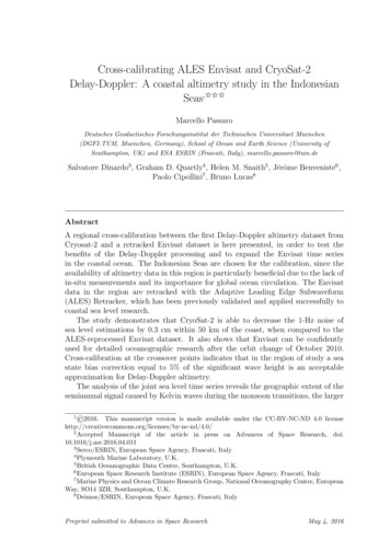
Cross-calibrating ALES Envisat and CryoSat-2Delay-Doppler: A coastal altimetry study in the IndonesianSeas,IIIMarcello PassaroDeutsches Geodaetisches Forschungsinstitut der Technischen Universitaet Muenchen(DGFI-TUM, Muenchen, Germany), School of Ocean and Earth Science (University ofSouthampton, UK) and ESA ESRIN (Frascati, Italy), marcello.passaro@tum.deSalvatore Dinardo3 , Graham D. Quartly4 , Helen M. Snaith5 , Jérôme Benveniste6 ,Paolo Cipollini7 , Bruno Lucas8AbstractA regional cross-calibration between the first Delay-Doppler altimetry dataset fromCryosat-2 and a retracked Envisat dataset is here presented, in order to test thebenefits of the Delay-Doppler processing and to expand the Envisat time seriesin the coastal ocean. The Indonesian Seas are chosen for the calibration, since theavailability of altimetry data in this region is particularly beneficial due to the lack ofin-situ measurements and its importance for global ocean circulation. The Envisatdata in the region are retracked with the Adaptive Leading Edge Subwaveform(ALES) Retracker, which has been previously validated and applied successfully tocoastal sea level research.The study demonstrates that CryoSat-2 is able to decrease the 1-Hz noise ofsea level estimations by 0.3 cm within 50 km of the coast, when compared to theALES-reprocessed Envisat dataset. It also shows that Envisat can be confidentlyused for detailed oceanographic research after the orbit change of October 2010.Cross-calibration at the crossover points indicates that in the region of study a seastate bias correction equal to 5% of the significant wave height is an acceptableapproximation for Delay-Doppler altimetry.The analysis of the joint sea level time series reveals the geographic extent of thesemiannual signal caused by Kelvin waves during the monsoon transitions, the larger 2016. This manuscript version is made available under the CC-BY-NC-ND 4.0 d/4.0/2Accepted Manuscript of the article in press on Advances of Space Research, doi:10.1016/j.asr.2016.04.0113Serco/ESRIN, European Space Agency, Frascati, Italy4Plymouth Marine Laboratory, U.K.5British Oceanographic Data Centre, Southampton, U.K.6European Space Research Institute (ESRIN), European Space Agency, Frascati, Italy7Marine Physics and Ocean Climate Research Group, National Oceanography Centre, EuropeanWay, SO14 3ZH, Southampton, U.K.8Deimos/ESRIN, European Space Agency, Frascati, Italy1Preprint submitted to Advances in Space ResearchMay 4, 2016
amplitudes of the annual signal due to the Java Coastal Current and the impact ofthe strong La Niña event of 2010 on rising sea level trends.Keywords: Coastal Altimetry; ALES; SAR altimetry; Indonesia; sea state bias;CryoSat-2; Envisat; SARvatore; sea level;1. IntroductionFor more than 20 years, studies of sea level and ocean topography have stronglyrelied on satellite altimetry. Standard altimeters work with a simple radar principle:signals are sent to the sea surface and the reflected echoes are registered onboardin time series called ”waveforms”. The pulse repetition frequency (PRF) of thesealtimeters is set in order to guarantee that the noise of consecutive echoes is uncorrelated (Walsh, 1982). This allows their incoherent processing: waveforms areaveraged in order to decrease the noise level. Subsequently, a model is fitted tothe averaged waveform (a process called ”retracking”) and the range (the distancebetween the satellite and the sea surface) is estimated.Standard altimeters achieve an accuracy of roughly 2-3 cm for 1-Hz averages(1 measurement every 7 km) (Bonnefond et al., 2011). Despite the remarkableperformance, data in the coastal zone are often disregarded due to land and calmwater interference in the satellite footprint (7.3 km for Envisat and 8.3 km forJason for calm seas (Quartly, 1998)) and degraded geophysical corrections. Theeffort of various research groups has led to a marked improvement in the retrievalof coastal sea level (Vignudelli et al., 2011). Among different coastal-dedicatedretracking techniques, the Adaptive Leading Edge Subwaveform (ALES) algorithmwas validated on 3 different missions against in-situ data, proving the possibility ofapplying the same method to both open-ocean and coastal data without degradingthe precision when compared to the standard products available (Passaro et al.,2014, 2015b).In order to improve the noise performance and reduce the footprint, the conceptof Delay-Doppler processing (also called ”SAR” processing) has been recently applied to radar altimetry. A Delay-Doppler altimeter is used on the CryoSat-2 (CS-2)mission and will be used on Sentinel-3. It sends pulses with a high PRF in order toachieve pulse-to-pulse coherence. Each resolution cell in the along-track direction ischaracterised by a Doppler frequency that can be exploited using the phase information of the complex echoes that return to the satellite. In this way, a higher numberof independent looks can be referred to a reduced footprint (pulse-Doppler limitedfootprint), which is effectively beam-limited ( 200 m in the along-track direction)when compared to the classic pulse-limited shape of the standard footprint (Raney,1998). CS-2 SAR ocean data have been locally validated against in-situ data andmodel data in the German Bight, showing improvements in precision compared tothe same data acquired with the pseudo low-resolution mode (PLRM) (FenoglioMarc et al., 2015).Both the ALES reprocessing of standard altimetry missions and the new SARaltimetry data should improve the sea level analysis in areas where satellite altimetryhas been previously disregarded. A previous study in the North Sea/Baltic Seaintersection zone, an area that is well-sampled by tide gauges, has shown that the2
ALES-based Envisat dataset has increased the amount and the quality of sea levelretrievals compared to other altimetry datasets, allowing a more accurate estimationof the annual cycle up to the coast (Passaro et al., 2015a). The use of CS-2 data(starting from 2010) should allow the extension of the Envisat time series (whichstopped in April 2012) in order to obtain a dense sampling of the ocean, moresuitable for regional analysis, when compared to the Jason series, whose groundtrack spacing at the equator is 315 km (7.5 km for CS-2, 90 km for Envisat).The aim of this paper is to inter-compare ALES-reprocessed Envisat and CS-2SAR sea level anomalies in the coastal ocean to: assess the performance of the SARaltimetry data; cross-calibrate the two missions to create multi-mission time-seriesand test the suitability of the dataset for sea level analysis on a basin-scale.The analysis is performed in the Indonesian Seas, an area that suffers from thelack of in-situ data despite being of key importance for climate dynamics and ahotspot for sea level rise. Despite the SAR data collection mode not being appliedeverywhere for CS-2, part of this area of study is included in a so called ”SAR box”.The two missions are inter-calibrated by means of crossover analysis. Compared tothe usual analysis of altimetric time series, this experiment is particularly challengingbecause of the orbit differences between the two satellites: Envisat had a 35-dayrepeat cycle, while CS-2 passes over the same ground-tracks once every 369 days,with 30-day sub-cycles.2. Area of studyThe Indonesian Seas act as a connection between the western Pacific Ocean andthe eastern Indian Ocean (figure 1) and as a key feature of the global ocean circulation: Their straits and passages form the Indonesian throughflow, which transportsnorth Pacific waters into the Indian Ocean.These waters enter the Indonesian throughflow primarily through the MakassarStrait (figure 2). Flowing south, the mass of water splits with one branch enteringthe Indian Ocean through the Lombok Strait and another flowing eastward throughthe Flores Sea and then through the Banda Sea, which has several narrow pathwaysthat lead the water into the Indian Ocean (Gordon, 2005).The interannual variability of the sea level anomalies in the area is dominated bythe El Niño Southern Oscillation. The annual cycle is driven by the monsoon winds,which blow from the west from November to March (northwest monsoon), and fromthe east from May to September (southeast monsoon).Rainfall increases over the whole area during the northwest monsoon. In the JavaSea, characterised by shallow depths, the northwest monsoon pushes low-salinitywater from the South China Sea up to the southern Makassar Strait, while highsalinity water from the Pacific Ocean enters the basin during the southeast monsoon(Durand and Petit, 2011). The reversal of the monsoon winds also inverts thedirection of the Java Coastal Current, which follows the bathymetry slope south ofthe island of Java (Syamsudin and Kaneko, 2013).Several studies have pointed out how the sea level in the south-east Asian regionis rising at rates higher than the global mean. In their study based on reconstructiontechniques to extend the altimetry analysis in time, Strassburg et al. (2014) have3
0 - 50 km50 - 100 km100 - 150 kmNorth Java24 m40 m46 mSouth Java757 m2623 m3397 mTable 1: Mean depth in relation to the distance from the coast in North Java andSouth Java.argued that the fast-rising sea level trends of the last two decades in the area maynot be the norm and could decrease with a weakening of the trade winds relatedto the phase of the Pacific Decadal Oscillation. This study and Palanisamy et al.(2015) found that trends increase from west to east in the geographical domain. Thealtimetry data which these studies rely on are gridded and interpolated, while ouranalysis is based on along-track data averaged according to the distance from thecoast. Results based on the interpolation of altimetry data that are not optimisedfor the coastal zone may cause gaps and lower quality of the measurements. At thesame time, given the highly populated coastal areas, it is beneficial to improve thequality of altimetry data in order to understand the dynamics of the sea level closeto the coast and on smaller scales.The use of local tide gauge sea level records is prevented by discontinuities and theinstability of the reference level due to strong vertical land movements, as shown byFenoglio-Marc et al. (2012). The availability of long and reliable satellite altimetryrecords could therefore help overcome the lack of in-situ data.Figure 1 shows the geographical limit of CS-2 SAR data and defines two domainsthat were selected North and South of Java Island (NJ and SJ from now on). Table1 shows the mean depth of NJ and SJ in relation to the distance from the coast,which is used as a criterion in the analysis of the next sections. The domains werechosen in order to contain both data from Envisat and from CS-2 SAR and to berepresentative of two very different conditions of a coastal ocean environment: inSJ, a strong coastal current with pronounced bathymetry slope characterised bymoderate waves and variability; in NJ, a shallow area with calmer sea state. Inthe crossover analysis (section 4.2) all the CS-2 SAR measurements included in thelatitude box of the map are taken into account.In section 4.3, time series of averaged cross-calibrated sea level measurementsare generated for the Java Sea, Flores Sea, Banda Sea, Bali Sea and Ceram Sea,defined according to the Limits of Ocean and Seas published by the InternationalHydrographic Organization in 1953 (see figure 2), despite the limited geographicalavailability of CS-2 SAR data. Figure 2 shows the extent of each of the IndonesianSeas.4
4oN0o4oS8oS99oE108oE117oE126oE135oE 10 100 200 300 400 500 1000 2000 3000 4000 5000Depth (m)8oNFigure 1: The domains selected North and South of Java Island (NJ and SJ) delimited by the black lines and the SAR boxes of CS-2 (delimited by the red lines).8 NMAKASSARSTRAIT4 NJavaMakassarBaliFloresBandaCeramBoni0 4 S8 SLOMBOKSTRAIT99 E108 E117 E126 E135 EFigure 2: The basins of interest within the Indonesian Seas, defined according to theLimits of Ocean and Seas published by the International Hydrographic Organizationin 1953.3. Data and Methods3.1. Altimetry DatasetThis study uses altimetry data from Envisat reprocessed with ALES and fromCS-2 SAR mode distributed with the ESA SAR Versatile Altimetric Toolkit forOcean and land Research and Exploitation (SARvatore) service. Envisat data coverorbital Phase B (from autumn 2002 to the 22nd October 2010) and orbital PhaseC (from 23rd October 2010 to 8th April 2012, after which contact with the satellitewas lost). During Phase C, Envisat was in an orbit 17.4 km lower than in Phase B,resulting in a slightly shorter repeat cycle of 30 days, and the overflight of different5
ground tracks. In this paper, when a distinction is needed, the two phases of Envisatwill be called Env B (Envisat Phase B) and Env C (Envisat Phase C).While over the vast majority of the ocean surface CS-2 operates in low resolutionmode (LRM), i.e. as a standard pulse-limited altimeter that does not exploit thepulse-to-pulse coherency, ”SAR” boxes are planned during the orbit, in particularwhen the satellite overpasses coastal oceans. Figure 1 shows that only a part of theIndonesian Seas is covered by a SAR box. Given the focus of this research and thecontent of the SARvatore product, only CS-2 SAR data are used in the analysis.SARvatore data were downloaded from gpod.eo.esa.int in May 2015. SARvatoreprocesses the CS-2 raw data in the SAR boxes using the SAMOSA2 functionalform (Ray et al., 2015); the settings suggested for coastal areas are all applied, i.e.Hamming weighting window on the burst data, zero-padding and extended radarreceiving window size (for details, see Dinardo and Benveniste (2013)).In order to harmonise the set of geophysical corrections applied to the rangemeasurement to derive the sea level height, the mean sea surface (MSS) from DTU13,the tidal amplitudes from DTU10 and the ECMWF-forced Dynamic AtmosphereCorrections are applied to both missions (for a justification of the choices, see Passaroet al. (2015a)). Concerning the Wet Tropospheric correction, given that CS-2 doesnot have a microwave radiometer on board, this study applies the ECMWF-basedcorrection to all the datasets.Based on what the available literature suggests for pulse-limited altimetry (Andersen and Scharroo, 2011), a tentative sea state bias (SSB) correction (still absentin the SARvatore product at the time of writing) is applied in this study, equal to4% of the SWH. An improvement of this tentative value is then proposed in section4.2.3.2. Data screening and outlier detectionALES Envisat 18-Hz sea level measurements were screened using the methodologyalready described in Passaro et al. (2015a). CS-2 data in SARvatore are distributedas 20-Hz and 1-Hz averages. In this study, 1-Hz points were recomputed startingfrom 20-Hz estimations using the same methodology as in Envisat, with the followingexceptions: The Coastal Proximity Parameter (CPP) parameter, which quantifies the influence of land on the radar returned echoes (Cipollini, 2011) and is used in the18-Hz data screening for Envisat, is not available for CS-2. Given the different footprint and antenna characteristics of CS-2, the Envisat CPP parametercannot be used; The fitting error in SARvatore is computed on the whole waveform and provided in waveform power units. A maximum value of 4 power units in thefitting error is adopted here, considering that analysis on open ocean datahas shown that 99% of the waveforms are fitted within this threshold (S.Dinardo, personal communication).The following additional screening was added on the 1-Hz points of both Envisatand CS-2 in order to exclude noisy retrievals, non-representative averages and errorsin the corrections. A 1-Hz point was excluded from the analysis if:6
The number of valid measurements within the 1-Hz block was less than 5. The standard deviation (std) of the valid measurements within the 1-Hz blockwas larger than 0.20 m; this criterion is justified by the fact that such a highslope in sea level would be not plausible in a distance of 7 km. The sum of the geophysical corrections, excluding ocean tides, was smallerthan 1 m; such values would be unrealistic given that, for example, the drytropospheric correction has a global mean of 2.31 m with only 2 cm std (Andersen and Scharroo, 2011).3.3. Methods for crossover analysisTo verify the precision and the agreement between Envisat and CS-2 SAR, acomparison of the sea level at the crossover points was performed. This is a standardpractice in altimetry and has been used is several publications as a key indicator ofthe data quality for altimetric missions (see Labroue et al. (2012) for a comprehensivelist of references). In order to reduce the impact of oceanic variability, crossovers aretaken into consideration if the time lag between the two passes is shorter than 10days. For most crossover analyses, coastal areas, shallow seas and high variabilityareas are generally avoided, while in this research they are explicitly taken intoconsideration. Crossovers are here defined as all the available 1-Hz points of twocrossing tracks that are closer than 5 km. Both Envisat and CS-2 measurementshave been referred to the same ellipsoid and the absolute bias found for Envisat(see Bonnefond et al. (2013)) was taken into account. Four crossover cases wereconsidered: Envisat Phase B ascending versus Envisat Phase B descending passes (caseEnvB-EnvB) Envisat Phase C ascending versus Envisat Phase C descending passes (caseEnvC-EnvC) Envisat Phase C ascending and descending versus CS-2 ascending and descending passes (case EnvC-CS2) CS-2 ascending versus CS-2 descending passes (case CS2-CS2)3.4. Regional derivation of seasonal signals and trends in the sea levelData were grouped depending on the corresponding basin and averaged everymonth. Given the stress in this study on the evaluation of coastal performances, datain NJ and SJ were divided according to distance from the coastline (0-50 km, 50-100km, 100-150 km). Estimations of annual and semiannual cycles were performed usingthe Prais Winsten Feasible Generalised Least Square Estimator, which accounts forthe problem of autocorrelation of the residuals in geophysical time series (Prais andWinsten, 1954). Subsequently, the seasonal cycle was removed from the time seriesand the trends were estimated using the same method.7
4. Results and discussion4.1. Comparison of performances between Envisat and CS-2In this section, the test areas of NJ and SJ are used for comparison of the performances of Envisat and CS-2, with particular focus on the coastal zone. The topplots of figure 3 show the number of passes for each month: the number of measurements available in the sub-basins in one month is similar in the time series ofboth missions. In two months of 2005 many passes of Envisat are missing and thisholds also for the initial 3 months after the launch of CS-2. In order to maintain theconsistency, for each mission statistics are shown only for months where more than10 passes are available.In order to check the consistency of the dataset, the middle plots of figure 3 showthe standard deviation of the retrieved SLA within 50 km of the coast. A singleaveraged sea level value for each pass of Envisat or CS-2 is assigned and each pointon the plot corresponds to the std considering all available passes in that month.The top plots show therefore the variability of the derived sea level (including errorsin the corrections) within a month in the domain of interest. The coastal regionof SJ has a higher variability than the corresponding area in NJ, as expected. Inboth regions, the average variability is consistent in all three missions: in SJ thereis an average monthly std of 9.2 cm for Env B, 10.0 cm for Env C and 9.5 cm forCS-2; in NJ the values are 7.0 cm for Env B, 7.8 cm for Env C and 7.2 for CS-2. Inthe 15 months when sufficient measurements were available from both Env C andCS-2, the root mean square difference between the monthly std from Env C andCS-2 is 2.4 cm in NJ and 1.8 cm in SJ. The retrieved variability is therefore verycomparable, despite the fact that the two satellites were sampling different areas ondifferent days. In SJ, all the months with a std exceeding 0.15 m are located in Mayor in November, i.e. during the expected onset of the monsoons.Figure 4 shows the monthly average of the 20 (18)-Hz SLA measurement noisecomputed at each 1-Hz location for CS-2 (Envisat) within 50 km of the coast. Inboth NJ and SJ, the average retrieved SWH is plotted in green for each mission.The noise level of Envisat is consistent between Phase B and Phase C. This helps tohighlight the differences between the sea state of the two areas and the relationshipbetween measurement noise and sea state, since higher SWH corresponds to noisierdata in all the datasets.A significant improvement in precision, when compared to Envisat, is remarkablein CS-2, whose noise is up to 1cm lower than for Env C in the same months for bothNJ and SJ. This result confirms that SAR altimetry is intrinsically more precisethan the standard processing. Although the validation of CS-2 SWH estimation isnot an objective of this research, it is remarkable that in both the areas CS-2 SWHis on average in very good agreement with the SWH measured by Env C.Figure 3 also shows the variability of the geophysical corrections, i.e. the sum ofwet (WTC) and dry tropospheric correction (DTC), dynamic atmosphere correction(DAC), ionospheric correction and sea state bias. Envisat and CS-2 data use thesame dataset for WTC, DTC and DAC. The std of the corrections applied to CS-2 isalmost double than that of Envisat. This difference is explained by considering theorbit of the satellites. Envisat follows a sun-synchronous orbit, therefore the satellite8
passes per month201002003 2005 2007 2009 2011 2013 2015monthly std (m)passes per monthmonthly std (m)North Java0.20.10South Java201002003 2005 2007 2009 2011 2013 2015ALES Env B 50Km from coastALES Env C 50Km from coastCS 2 50 Km from coast0.20.102003 2005 2007 2009 2011 2013 2015geo.corr. monthly std (m)geo.corr. monthly std (m)2003 2005 2007 2009 2011 2013 20150.20.102003 2005 2007 2009 2011 2013 20150.20.102003 2005 2007 2009 2011 2013 2015Figure 3: Top: number of satellite passes available in each month. Middle: StandardDeviation of the monthly SLA values in SJ and NJ within 50 km of the coast for EnvB ALES (blue), Env C ALES (orange) and CryoSat-2 SARvatore (red). Only datafrom months when at least 10 passes were available are shown. Bottom: StandardDeviation of the monthly geophysical correction applied to the SLA estimations.flies over the same area at the same time of day. This is not true for CS-2, as it isshown in figure 5: depending on ascending and descending orbits, Envisat overpassesthe area in two clearly defined sections of the day, while the measurements of CS-2span the whole 24 hours. In fact, all the geophysical effects have their own diurnalcycle linked to the daily variation of the atmospheric pressure (Ponte and Ray, 2002),ionospheric electron content (Liu et al., 2011) and wet and dry component in thetroposphere (Jin et al., 2009).Tables 2 and 3 show the consistency of noise and variability w.r.t. the distancefrom the coast in NJ and SJ, by averaging in time the previous statistics. In bothNJ and SJ, the difference in variability between the different missions is always lessthan 1.5 cm. This is particularly important considering that both Env C and CS-2sample areas that were not sampled by previous missions, whose data are used tobuild the MSS models.Compared to figure 4, the noise in the tables is scaled at 1Hz level, i.e. the highrate noise is divided by the root mean square of the number of measurements in each1 Hz block. The data confirm the robustness of the improvement in precision broughtby CS-2, quantifiable as roughly 0.3 cm at 1 Hz level w.r.t. Envisat regardless ofthe sea state.9
NORTH JAVAMonthly std1-Hz noiseAlt data set0 - 50 km50 - 100 km100 - 150 kmALES Env B7.1 cm7.2 cm6.4 cmALES Env C7.8 cm7.4 cm7.7 cmCS-27.2 cm6.9 cm6.6 cmALES Env B1.2 cm1.1 cm1.2 cmALES Env C1.2 cm1.2 cm1.2 cmCS-20.9 cm0.8 cm0.8 cmTable 2: Variability of the parameters of interest (standard deviation of the monthlySLA values and average 1-Hz noise of the SLA values) in North Java depending onthe distance from the coastline for Env B ALES, Env C ALES and CS-2 SARvatore.SOUTH JAVAMonthly std1-Hz noiseAlt data set0 - 50 km50 - 100 km100 - 150 kmALES Env B9.2 cm8.0 cm7.8 cmALES Env C10.0 cm9.5 cm9.0 cmCS-29.5 cm8.2 cm8.7 cmALES Env B1.7 cm1.6 cm1.6 cmALES Env C1.7 cm1.6 cm1.6 cmCS-21.4 cm1.3 cm1.3 cmTable 3: Variability of the parameters of interest (standard deviation of the monthlySLA values and average 1-Hz noise of the SLA values) in South Java depending onthe distance from the coastline for Env B ALES, Env C ALES and CS-2 SARvatore.10
430.0420.02SWH e 4: Average 20Hz noise of the SLA values in SJ and NJ within 50 km of thecoast for Env B ALES (blue), Env C ALES (orange) and CS-2 SARvatore (red).Also shown is the average estimated Significant Wave Height for each mission (greencurves)30EnvisatCryosat 2% of measurements2520151050051015Hour of overpass (UTC)2025Figure 5: Overpass time in the Java region for Envisat (blue) and CryoSat-2 (red).4.2. Crossover analysis and cross-calibrationIn this section, the analysis of the crossovers in the test areas of NJ and SJ isdiscussed, in order to cross-calibrate the two missions. Figure 6 shows the charac11SWH (m)North Java 20Hz noise (m)South Java 20Hz noise (m)5ALES Env B 50Km from coastALES Env C C 50Km from coastCS 2 50 Km from coast0.08
Crossover difference (m)teristics of the crossovers for each case in terms of time lag and distance from thecoast. While crossovers in case EnvC-CS2 span the whole 10 days of permitted timedifference, all the other cases, due to the orbit characteristics, are bounded to specifictime lags that are latitude dependant. In terms of distance from the coastline, validcase CS2-CS2 crossovers were found only further than 70 km from the coast, whileall the other cases were representative of both coastal and open ocean conditions.Whilst the mono-mission crossovers lie in discrete latitudinal bands ( 9.8 S forCS2-CS2, 9.8 , 8.2 & 4.8 S for EnvB-EnvB, and 8.6 & 6.7 S for EnvC-EnvC), theEnvC-CS2 crossovers occur at all latitudes (not shown), corresponding to the fullrange of distances from the coast and the full range of time separations. This alsomeans that the phase difference of any error in a component of the tide model isfairly evenly spread over [0,2π] and thus tidal uncertainties will produce no meanoffset between the two SLA datasets.EnvC CS2CS2 CS2EnvB EnvBEnvC EnvC10.50 0.5 1012345678910Time difference (days)Crossover difference (m)10.50 0.5 1050100150200250Distance from coast (km)Figure 6: Upper plot: distribution of crossover differences depending on time difference between the satellite passes. Lower plot: distribution of crossover differencesdepending on distance from the coastline.In order to have a fair comparison, the histogram on the left of figure 7 comparesthe four cases considering only points located further than 70 km from the coast.Performances for different missions are extremely similar and unbiased, since themean of the crossover differences is zero. Concerning mono-mission crossovers, thesmall differences in the histogram of case CS2-CS2 compared to EnvB-EnvB andEnvC-EnvC correspond to the time differences of the crossovers seen in figure 6.Concerning the case EnvC-CS2, the crossover differences have a mean of 1.4 cm,which goes down to -0.6 cm when considering the crossover differences withoutapplying any SSB correction to either of the two missions (black histogram in the12
plot on the right). The mean of the crossover differences is considerably lower thanthe global mean difference found by (Labroue et al., 2012) between Env B and CS-2LRM mode crossovers (5.8 cm), which considered only one month of data and onlydeep water and low variability region.2525EnvC CS2CS2 CS2EnvB EnvBEnvC EnvCEnvC CS2EnvC CS2 [NO SSB]20Percentage of crossoversPercentage of crossovers2015105151050 0.5 0.4 0.3 0.2 0.1 0 0.1 0.2 0.3 0.4Crossover difference (m)0 0.5 0.4 0.3 0.2 0.1 0 0.1 0.2 0.3 0.4Crossover difference (m)0.50.5Figure 7: Left: Histogram of crossover differences considering only points fartherthan 70 km of the coast. Right: Same histogram with focus on the crossovers betweenEnv C and CS-2 with and without applying a SSB correction to each dataset.A clearer evaluation that considers both coastal and open ocean conditions isfound in figure 8. The plots focus on the coastal zone, showing the statistics between0 and 25 km and between 25 and 50 km from the coast, considering as ”open ocean”anything beyond 50 km. Statistics for the case CS2-CS2 in the coastal zone arenot presented due to the lack of coastal crossovers in the area of study for CS-2.The upper plot shows the mean of the crossover differences. The cases of the samemission are centred on zero within half a cm. The EnvC-CS2 comparison shows abias slightly higher than 1 cm in the area closest to the coast and in the open ocean.The standard deviation of the crossover differences is about 10 cm for all cases inthe open ocean; it increases in the coastal zone, but is always less than 15 cm (figure8, middle plot).An analysis of the SLA differences at the EnvC-CS2 crossovers w.r.t. the SWHestimated by CS-2 is shown in figure 9 for NJ and SJ. The difference of wave conditions encountered in the two test regions is immediately visible: NJ never encountersa SWH higher than 2 m in the observ
repeat cycle, while CS-2 passes over the same ground-tracks once every 369 days, with 30-day sub-cycles. 2. Area of study The Indonesian Seas act as a connection between the western Paci c Ocean and the eastern Indian Ocean ( gure 1) and as a key feature of the global ocean circula-tion: Their straits and passages form the Indonesian through