WIXLIB

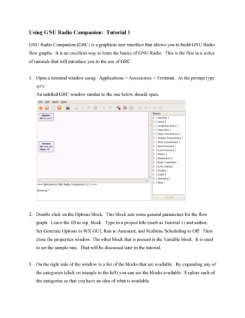
Using GNU Radio Companion: Tutorial 1GNU Radio Companion (GRC) is a graphical user interface that allows you to build GNU Radioflow graphs. It is an excellent way to learn the basics of GNU Radio. This is the first in a seriesof tutorials that will introduce you to the use of GRC.1. Open a terminal window using: Applications Accessories Terminal. At the prompt type:grcAn untitled GRC window similar to the one below should open.2. Double click on the Options block. This block sets some general parameters for the flowgraph. Leave the ID as top block. Type in a project title (such as Tutorial 1) and author.Set Generate Options to WX GUI, Run to Autostart, and Realtime Scheduling to Off. Thenclose the properties window. The other block that is present is the Variable block. It is usedto set the sample rate. That will be discussed later in the tutorial.3. On the right side of the window is a list of the blocks that are available. By expanding any ofthe categories (click on triangle to the left) you can see the blocks available. Explore each ofthe categories so that you have an idea of what is available.

4. Open the Sources category and double click on the Signal Source. Note that a Signal Sourceblock will now appear in the main window. Double click on the block and the propertieswindow will open. Adjust the settings to match those as shown in the figure below and closethe window. This Signal Source is now set to output a real valued 1KHz sinusoid with anamplitude of .5.5. In order to view this wave we need one of the graphical sinks. Expand the Graphical Sinkcategory and double click on the Scope Sink. It should appear in the main window. Doubleclick on the block and change the Type to Float. Leave the other Parameters at their defaultvalues and close the properties window.6. In order to connect these two blocks, click once on the “out” port of the Signal Source, andthen once on the “in” port of the Scope Sink. The following flow graph should be displayed.

7. You may have noticed a warning in the message window indicating that the flow graph maynot have flow control. Add a Throttle block between the source and the sink as shown in thefigure below. Make sure to change the Throttle Type to Float. Note that before you do that,the Generate flow graph icon cannot be selected. This is because there is an error in the flowgraph. Generate and execute the flow graph to confirm that it still works.8. In order to observe the operation of this simple system we must generate the flow graph andthen execute it. Click first on the “Generate the flow graph” icon. A box will come up inwhich you enter the name of the file. Name this file: tutorial1.grc and save.

9. Click the “Execute the flow graph” icon. A scope plot should open displaying several cyclesof the sinusoid. Confirm that the frequency and amplitude match the value that you expect.Experiment with the controls on the scope plot.10. Change the Channel Options, Marker setting to Dot Large. Now you can see the actualsample values. Recall that the Variable block set the sampling rate to 32000 samples/secondor 32 samples/ms. Note that there are in fact 32 samples within one cycle of the wave.11. Close the Scope Plot and reduce the sample rate to 10000 by double clicking on the Variableblock. Re-generate and execute the flow graph. Note that there are now fewer points percycle. How low can you drop the sample rate? Recall that the Nyquist sampling theoremrequires that we sample at more than two times the highest frequency. Experiment with thisand see how the output changes as you drop below the Nyquist rate.12. Close the Scope Plot and change the sample rate back to 32000. Add an FFT Sink (underGraphical Sinks) to your window. Change the Type to Float and leave the remainingparameters at their default values.13. Connect this to the output of the Signal Source by clicking on the out port of the SignalSource and then the in port of the FFT Sink. Generate and execute the flow graph. Youshould observe the scope as before along with an FFT plot correctly showing the frequencyof the input at 1KHz. Close the output windows.14. Explore the other Graphical Sinks (Number Sink, Waterfall Sink, and Histo Sink) to see howthey display the Signal Source.15. Create the flow graph shown below. The Audio Sink is found in the Sinks category.Generate and execute the flow graph. The graphical display of the scope and FFT shouldopen as before. However, now you should also hear the 1KHz tone. The Audio Sink block

directs the signal to the audio card of your computer. Depending on the sampling rate of theaudio card in your computer, you may get an error message in the GRC message window:Audio alsa sink[hw:0,0]: unable to support sampling rate32000, card requested 44100 instead.If you do see a message similar to this, stop the execution and double click on the variableblock to change the sample rate to 44100 (or whatever your error message indicates).Generate and execute the flow graph again and the error message should be gone.16. Construct the flow graph shown below. Set the sample rate to 32000. The two SignalSources should have frequencies of 1000 and 800, respectively. The Add block is found inthe Operators category.

17. Generate and execute the flow graph. On the Scope plot you should observe a waveformcorresponding to the sum of two sinusoids. On the FFT plot you should see components atboth 800 and 1000 Hz. Unfortunately, the FFT plot does not provide enough resolution toclearly see the two distinct components. Note that the maximum frequency displayed on thisplot is 16KHz. This is one-half of the 32KHz sample rate. In order to obtain betterresolution, we can lower the sample rate. Try lowering the sample rate to 10KHz.18. Replace the Add block with a Multiply block. What output do you expect from the productof two sinusoids? Confirm your result on the Scope and FFT displays.19. Modify the flow graph to include a Low Pass Filter block as shown in the figure below. Thisblock is found in the Filters category and is the first Low Pass Filter listed. Recall that theMultiply block outputs a 200Hz and a 1.8KHz sinusoid. We want to create a filter that willpass the 200Hz and block the 1.8KHz component. Set the low pass filter to have a cutofffrequency of 1KHz and a transition width of 200 Hz. Use a Rectangular Window. Generateand execute the flow graph. You should observe that only the 200Hz component passesthrough the filter. Experiment with the High Pass Filter.

20. Using the same flow graph, change the sample rate variable to 20000. Change theDecimation in the Low Pass Filter to 2. Decimation decreases the number of samples thatare processed. A decimation factor of two means that the output of the filter will have asample rate equal to one-half of the input sample rate, or in this case only 10000 samples/sec.This is a sufficient sample rate for the frequencies that we are dealing with. Generate andexecute the flow graph. What frequency do you observe on the FFT? Measure it preciselyby letting the cursor hover over the peak of the observed component.21. You should have observed that the FFT is now measuring a signal around 400 Hz, rather thanthe expected 200Hz. Why is this error occurring? It is because the sample rate on the FFThas not been adjusted to properly measure its input. Double click on the FFT Sink block andchange the sample rate to samp rate/2. Generate and execute the flow graph. You shouldnow read the correct frequency.

22. Open a file browser in Ubuntu (Places Home Folder). Go to the directory that containsthe GRC file that you have been working on. If you are unsure as to where this is, the path tothis file is shown in the bottom portion of the GRC window. In addition to saving a “.grc”file with your flow graph, note that there is also a file titled “top block.py”. Double click onthis block. You will be given the option to Run or Display this file. Select Display. This isthe Python file that is generated by GRC. It is this file that is being run when you execute theflow graph. You can modify this file and run it from the terminal window. This allows youto use features that are not included in GRC. Keep in mind that every time you run your flowgraph in GRC, it will overwrite the Python script that is generated. So, if you make changesdirectly in the Python script that you want to keep, save it under another name.

graph. Leave the ID as top_block. Type in a project title (such as Tutorial 1) and author. Set Generate Options to WX GUI, Run to Autostart, and Realtime Scheduling to Off. Then close the properties window. The other block that is present is the Variable block. It is used to set the sample rate. That will be discussed later in the tutorial. 3.