WIXLIB

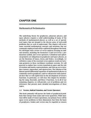
Mathematical Methods in Engineering and ScienceBasisOperational Fundamentals of Linear AlgebraRange and Null Space: Rank and NullityBasisChange of BasisElementary TransformationsTake a set of vectors v1 , v2 , · · · , vr in a vector space.Question: Given a vector v in the vector space, can we describe itasv k1 v1 k2 v2 · · · kr vr Vk,where V [v1 v2 · · · vr ] and k [k1 k2 · · · kr ]T ?Answer: Not necessarily.Span, denoted as v1 , v2 , · · · , vr : the subspacedescribed/generated by a set of vectors.Basis:A basis of a vector space is composed of an orderedminimal set of vectors spanning the entire space.The basis for an n-dimensional space will have exactly nmembers, all linearly independent.29,

Mathematical Methods in Engineering and ScienceOperational Fundamentals of Linear AlgebraBasisRange and Null Space: Rank and NullityBasisChange of BasisElementary TransformationsOrthogonal basis: {v1 , v2 , · · · , vn } withOrthonormal basis:vjT vkvjT vk 0 j 6 k. δjk 01ififj 6 kj kMembers of an orthonormal basis form an orthogonal matrix.Properties of an orthogonal matrix:V 1 VT or VVT I, andNatural basis: e1 det V 1 or 1,100.0 , e2 010.0 , ··· , en 000.1 . 30,

Mathematical Methods in Engineering and ScienceOperational Fundamentals of Linear AlgebraChange of BasisRange and Null Space: Rank and NullityBasisChange of BasisnElementary TransformationsSuppose x represents a vector (point) in R in some basis.Question: If we change over to a new basis {c1 , c2 , · · · , cn }, howdoes the representation of a vector change?x x̄1 c1 x̄2 c2 · · · x̄n cn x̄1 x̄2 [c1 c2 · · · cn ] . . . x̄nWith C [c1c2···cn ],new to old coordinates: Cx̄ x andold to new coordinates: x̄ C 1 x.Note: Matrix C is invertible. How?Special case with C orthogonal:orthogonal coordinate transformation.31,

Mathematical Methods in Engineering and ScienceOperational Fundamentals of Linear AlgebraChange of BasisRange and Null Space: Rank and NullityBasisChange of BasisElementary TransformationsQuestion: And, how does basis change affect the representation ofa linear transformation?A : R n R m,Consider the mappingAx y.Change the basis of the domain through P R n n and that of theco-domain through Q R m m .New and old vector representations are related asPx̄ xandQȳ y.Then, Ax y Āx̄ ȳ, withĀ Q 1 APSpecial case: m n and P Q gives a similarity transformationĀ P 1 AP32,

Mathematical Methods in Engineering and ScienceElementary TransformationsOperational Fundamentals of Linear AlgebraRange and Null Space: Rank and NullityBasisChange of BasisElementary TransformationsObservation: Certain reorganizations of equations in a systemhave no effect on the solution(s).Elementary Row Transformations:1. interchange of two rows,2. scaling of a row, and3. addition of a scalar multiple of a row to another.Elementary Column Transformations: Similar operations withcolumns, equivalent to a corresponding shuffling of the variables(unknowns).33,

Mathematical Methods in Engineering and ScienceOperational Fundamentals of Linear AlgebraElementary TransformationsRange and Null Space: Rank and NullityBasisChange of BasisElementary TransformationsEquivalence of matrices: An elementary transformation definesan equivalence relation between two matrices.Reduction to normal form:AN Ir000 Rank invariance: Elementary transformations do not alter therank of a matrix.Elementary transformation as matrix multiplication:an elementary row transformation on a matrix isequivalent to a pre-multiplication with an elementarymatrix, obtained through the same row transformation onthe identity matrix (of appropriate size).Similarly, an elementary column transformation is equivalent topost-multiplication with the corresponding elementary matrix.34,

Mathematical Methods in Engineering and SciencePoints to noteOperational Fundamentals of Linear AlgebraRange and Null Space: Rank and NullityBasisChange of BasisElementary Transformations Concepts of range and null space of a linear transformation. Effects of change of basis on representations of vectors andlinear transformations. Elementary transformations as tools to modify (simplify)systems of (simultaneous) linear equations.Necessary Exercises: 2,4,5,635,

Mathematical Methods in Engineering and ScienceOutlineSystems of Linear EquationsNature of SolutionsBasic Idea of Solution MethodologyHomogeneous SystemsPivotingPartitioning and Block OperationsSystems of Linear EquationsNature of SolutionsBasic Idea of Solution MethodologyHomogeneous SystemsPivotingPartitioning and Block Operations36,

Mathematical Methods in Engineering and ScienceSystems of Linear EquationsNature of SolutionsNature of SolutionsBasic Idea of Solution MethodologyHomogeneous SystemsPivotingPartitioning and Block OperationsAx bCoefficient matrix: A, augmented matrix: [A b].Existence of solutions or consistency:Ax bhas a solution b Range(A) Rank(A) Rank([A b])Uniqueness of solutions:Rank(A) Rank([A b]) nSolution of Ax b is unique. Ax 0 has only the trivial (zero) solution.Infinite solutions: For Rank(A) Rank([A b]) k n, solutionx x̄ xN ,with Ax̄ bandxN Null (A)37,

Mathematical Methods in Engineering and ScienceSystems of Linear EquationsBasic Idea of Solution MethodologyTo diagnoseNature of SolutionsBasic Idea of Solution MethodologyHomogeneous SystemsPivotingPartitioning and Block Operationsthe non-existence of a solution,To determine the unique solution, orTo describeinfinite solutions;decouple the equations using elementary transformations.For solving Ax b, apply suitable elementary row transformationson both sides, leading toRq Rq 1 · · · R2 R1 Ax Rq Rq 1 · · · R2 R1 b,or,[RA]x Rb;such that matrix [RA] is greatly simplified.In the best case, with complete reduction, RA In , andcomponents of x can be read off from Rb.For inverting matrix A, treat AA 1 In similarly.38,

Mathematical Methods in Engineering and ScienceHomogeneous SystemsSystems of Linear EquationsNature of SolutionsBasic Idea of Solution MethodologyHomogeneous SystemsPivotingPartitioning and Block OperationsTo solve Ax 0 or to describe Null (A),apply a series of elementary row transformations on A to reduce it to the A,the row-reduced echelon form or RREF.Features of RREF:1. The first non-zero entry in any row is a ‘1’, the leading ‘1’.2. In the same column as the leading ‘1’, other entries are zero.3. Non-zero entries in a lower row appear later.Variables corresponding to columns having leading ‘1’sare expressed in terms of the remaining variables. u1 u2 Solution of Ax 0: x z1 z2 · · · zn k ··· un kBasis of Null(A): {z1 , z2 , · · · , zn k }39,

Mathematical Methods in Engineering and SciencePivotingSystems of Linear EquationsNature of SolutionsBasic Idea of Solution MethodologyHomogeneous SystemsPivotingPartitioning and Block OperationsAttempt:To get ‘1’ at diagonal (or leading) position, with ‘0’ elsewhere.Key step: division by the diagonal (or leading) entry.Consider Ik. . . .δ . . . . . BIG . .Ā .big. . . . . . .Cannot divide by zero. Should not divide by δ. partial pivoting: row interchange to get ‘big’ in place of δ complete pivoting: row and column interchanges to get‘BIG’ in place of δComplete pivoting does not give a huge advantage over partial pivoting,but requires maintaining of variable permutation for later unscrambling.40,

Mathematical Methods in Engineering and SciencePartitioning and Block OperationsSystems of Linear EquationsNature of SolutionsBasic Idea of Solution MethodologyHomogeneous SystemsPivotingPartitioning and Block OperationsEquation Ax y can be written as x1 A11 A12 A13 y1x2 ,A21 A22 A23y2x3with x1 , x2 etc being themselves vectors (or matrices). For a valid partitioning, block sizes should be consistent. Elementary transformations can be applied over blocks. Block operations can be computationally economical at times. Conceptually, different blocks of contributions/equations canbe assembled for mathematical modelling of complicatedcoupled systems.41,

Mathematical Methods in Engineering and SciencePoints to noteSystems of Linear EquationsNature of SolutionsBasic Idea of Solution MethodologyHomogeneous SystemsPivotingPartitioning and Block Operations Solution(s) of Ax b may be non-existent, unique orinfinitely many. Complete solution can be described by composing a particularsolution with the null space of A. Null space basis can be obtained conveniently from therow-reduced echelon form of A. For a strategy of solution, pivoting is an important step.Necessary Exercises: 1,2,4,5,742,

Mathematical Methods in Engineering and ScienceOutlineGauss Elimination Family of MethodsGauss-Jordan EliminationGaussian Elimination with Back-SubstitutionLU DecompositionGauss Elimination Family of MethodsGauss-Jordan EliminationGaussian Elimination with Back-SubstitutionLU Decomposition43,

Mathematical Methods in Engineering and ScienceGauss Elimination Family of MethodsGauss-Jordan EliminationGauss-Jordan EliminationGaussian Elimination with Back-SubstitutionLU DecompositionTask: Solve Ax b1 , Ax b2 and Ax b3 ; find A 1 andevaluate A 1 B, where A R n n and B R n p .Assemble C [A b1 b2and follow the algorithm .b3InB] R n (2n 3 p)Collect solutions from the result C C [InA 1 b1A 1 b2A 1 b3A 1A 1 B].Remarks: Premature termination: matrix A singular — decision? If you use complete pivoting, unscramble permutation. Identity matrix in both C and C? Store A 1 ‘in place’. For evaluating A 1 b, do not develop A 1 . Gauss-Jordan elimination an overkill? Want somethingcheaper ?44,

Mathematical Methods in Engineering and ScienceGauss Elimination Family of MethodsGauss-Jordan EliminationGauss-Jordan EliminationGaussian Elimination with Back-SubstitutionLU DecompositionGauss-Jordan Algorithm 1For k 1, 2, 3, · · · , (n 1)1. Pivot : identify l such that clk max cjk for k j n.If clk 0, then 0 and exit.Else, interchange row k and row l.2. ckk ,Divide row k by ckk .3. Subtract cjk times row k from row j, j 6 k. cnn If cnn 0, then exit.Else, divide row n by cnn .In case of non-singular A,default termination .This outline is for partial pivoting.45,

Mathematical Methods in Engineering and ScienceGauss Elimination Family of MethodsGauss-Jordan EliminationGaussian Elimination with Back-SubstitutionGaussian Elimination with Back-SubstitutionLU DecompositionGaussian elimination:Ax b ′′a11a12···′ a22 · · · or, . . Back-substitutions: Ax b ′ ′b1x1a1n′ ′ x a2n b2 2 . . . . . . ′xnbn′ann′xn bn′ /ann, nX1 ′xi aij′ xj for i n 1, n 2, · · · , 2, 1bi aii′j i 1Remarks Computational cost half compared to G-J elimination. Like G-J elimination, prior knowledge of RHS needed.46,

Mathematical Methods in Engineering and ScienceGauss Elimination Family of MethodsGauss-Jordan EliminationGaussian Elimination with Back-SubstitutionGaussian Elimination with Back-SubstitutionLU DecompositionAnatomy of the Gaussian elimination:The process of Gaussian elimination (with no pivoting) leads toU Rq Rq 1 · · · R2 R1 A RA.The steps given byfor k 1, 2, 3, · · · , (n 1)j-th row j-th row j k 1, k 2, · · · , ninvolve elementary matrices Rk k 1With L R 1 , 1 aa2111 aa3111. aan111A LU.ajkakk 0 0 ···1 0 ···0 1 ···. . . . .0 0 ···k-th row000.1 etc. for47,

Mathematical Methods in Engineering and ScienceGauss Elimination Family of MethodsLU DecompositionGauss-Jordan EliminationGaussian Elimination with Back-SubstitutionLU DecompositionA square matrix with non-zero leading minors is LU-decomposable.No reference to a right-hand-side (RHS) vector!To solve Ax b, denote y Ux and split asAx b LUx b Ly bForward substitutions: i 1X1lij yj yi bi liij 1Back-substitutions: nX1 uij xj yi xi uiij i 1andUx y.for i 1, 2, 3, · · · , n;for i n, n 1, n 2, · · · , 1.48,

Mathematical Methods in Engineering and ScienceGauss Elimination Family of MethodsLU Decomposition49,Gauss-Jordan EliminationGaussian Elimination with Back-SubstitutionLU DecompositionQuestion: How to LU-decompose a given matrix? L l11l21l31.000l22l32.l33.ln1ln2ln3 ·········.000.···lnn and U 3n.000···unnElements of the product giveiXandk 1jXlik ukj aijfor i j,lik ukj aijfor i j.k 1n2 equations in n2 n unknowns: choice of n unknowns

Mathematical Methods in Engineering and ScienceLU DecompositionGauss Elimination Family of MethodsGauss-Jordan EliminationGaussian Elimination with Back-SubstitutionLU DecompositionDoolittle’s algorithm Choose lii 1For j 1, 2, 3, · · · , nPi 11. uij aij k 1lik ukj for 1 i jPj 112. lij ujj (aij k 1 lik ukj ) for i jEvaluation proceeds in column order of u11 u12 u13 l21 u22 u23 A l31 l32 u33 . .ln1 ln2 ln3the matrix (for storage) · · · u1n· · · u2n · · · u3n . . · · · unn50,

Mathematical Methods in Engineering and ScienceGauss Elimination Family of MethodsLU DecompositionGauss-Jordan EliminationGaussian Elimination with Back-SubstitutionLU DecompositionQuestion: What about matrices which are not LU-decomposable?Question: What about pivoting?Consider the non-singular matrix 0 1 210 0u11 0 u12 u13 3 1 2 l21 ? 1 0 0u22 u23 .2 1 3l31l32 100 u33LU-decompose a permutation of its rows 0 32 1 21 2 1 3 0 10 0 10 1 00 0 0 1 1 00 0 0 1 1 21 2 1 3 1 0 03 10 1 0 0 1120 0133302 22 .1In this PLU decomposition, permutation P is recorded in a vector.51,

Mathematical Methods in Engineering and SciencePoints to noteGauss Elimination Family of MethodsGauss-Jordan EliminationGaussian Elimination with Back-SubstitutionLU DecompositionFor invertible coefficient matrices, use Gauss-Jordan elimination for large number of RHS vectorsavailable all together and also for matrix inversion, Gaussian elimination with back-substitution for small numberof RHS vectors available together, LU decomposition method to develop and maintain factors tobe used as and when RHS vectors are available.Pivoting is almost necessary (without further special structure).Necessary Exercises: 1,4,552,

Mathematical Methods in Engineering and ScienceOutlineSpecial Systems and Special Methods53,Quadratic Forms, Symmetry and Positive DefinitenesCholesky DecompositionSparse Systems*Special Systems and Special MethodsQuadratic Forms, Symmetry and Positive DefinitenessCholesky DecompositionSparse Systems*

Mathematical Methods in Engineering and ScienceSpecial Systems and Special Methods54,Quadratic Forms, Symmetry and Positive DefinitenesQuadratic Forms, Symmetry and PositiveDefinitenessCholesky DecompositionSparse Systems*Quadratic formTq(x) x Ax nn XXaij xi xji 1 j 1defined with respect to a symmetric matrix.Quadratic form q(x), equivalently matrix A, is called positivedefinite (p.d.) whenxT Ax 0 x 6 0and positive semi-definite (p.s.d.) whenxT Ax 0 x 6 0.Sylvester’s criteria:a11 0,a11 a12a21 a22 0, · · · , det A 0;i.e. all leading minors non-negative, for p.s.d.

Mathematical Methods in Engineering and ScienceSpecial Systems and Special MethodsCholesky Decomposition55,Quadratic Forms, Symmetry and Positive DefinitenesCholesky DecompositionSparse Systems*If A R n n is symmetric and positive definite, then there exists anon-singular lower triangular matrix L R n n such thatA LLT .Algorithm For i 1, 2, 3, · · · , nqP 1 2 Lii aii ik 1Lik Pi 1 Lji 1 aji LLjkikk 1Liifor i j nFor solving Ax b,Forward substitutions: Ly bBack-substitutions: LT x yRemarks Test of positive definiteness. Stable algorithm: no pivoting necessary! Economy of space and time.

Mathematical Methods in Engineering and ScienceSparse Systems* What is a sparse matrix? Bandedness and bandwidth Efficient storage and processingUpdates Sherman-Morrison formula(A uvT ) 1 A 1 Special Systems and Special Methods(A 1 u)(vT A 1 )1 vT A 1 uWoodbury formulaConjugate gradient method 56,Quadratic Forms, Symmetry and Positive DefinitenesCholesky DecompositionSparse Systems*efficiently implemented matrix-vector products

Mathematical Methods in Engineering and SciencePoints to noteSpecial Systems and Special Methods Concepts and criteria of positive definiteness and positivesemi-definiteness Cholesky decomposition method in symmetric positive definitesystems Nature of sparsity and its exploitationNecessary Exercises: 1,2,4,757,Quadratic Forms, Symmetry and Positive DefinitenesCholesky DecompositionSparse Systems*

Mathematical Methods in Engineering and ScienceOutlineNumerical Aspects in Linear SystemsNorms and Condition NumbersIll-conditioning and SensitivityRectangular SystemsSingularity-Robust SolutionsIterative MethodsNumerical Aspects in Linear SystemsNorms and Condition NumbersIll-conditioning and SensitivityRectangular SystemsSingularity-Robust SolutionsIterative Methods58,

Mathematical Methods in Engineering and ScienceNumerical Aspects in Linear SystemsNorms and Condition NumbersNorm of a vector: a measure of sizeNorms and Condition NumbersIll-conditio

Geometry and Algebra Linear Transformations Matrix Terminology Geometry and Algebra Let vector x [x 1 x 2 x 3]T denote a point (x 1,x 2,x 3) in 3-dimensional space in frame of reference OX 1X 2X 3. Example: With m 2 and n 3, y 1 a 11x 1 a 12x 2 a 13x 3 y 2 a 21x 1 a 22x 2 a 23x 3 . Plot y 1 and y 2 in the OY 1Y 2 plane. 1 R 2 X .