WIXLIB

11/14/19Multivariate Calculus: Vector CalculusHavenscoordinates (x, y, z), one has:Dı̂ , xD ̂ , yDk̂ . zProposition 1.1. The directional derivative of f in the direction of û at a point r0 D may becalculated asnX f(r0 ) ,Dû f (r0 ) ui xii 1where ui are the components of û in rectangular coordinates on Rn and xi are the n variables of fgiving the rectangular coordinates of a general vector argument r.Proof. This is a straightforward consequence of the multivariate chain rule – see (1). Several natural questions arise immediately: For a fixed point r0 D, can one readily determine for what û Sn 1 the directionalderivative Dû f (r0 ) is largest? That is, how do we determine the direction leaving r0 thatmaximizes the rate of change of the function f ? What can be said about directions in which the directional derivative vanishes? Is there a coordinate free and geometric way to understand the directional derivative operator, other than its defining limit formula? That is, as the formula above to calculate it isnot coordinate independent, can we instead describe the directional derivative operator in ageometric way that doesn’t invoke rectangular coordinates, or some other arbitrary choice?After all, the directional derivative “frees us” from considering only the way f changesalong coordinate directions, and its limit definition suggests that it lives independently ofcoordinates.Observe that the expression in the theorem is reminiscent of the formula for a dot product interms of the components of two vectors in rectangular coordinates. Indeed, we shall realize it assuch–we will momentarily define the gradient of f at r0 to be a vector which fulfills the necessary roleto allow us to view this computation as being a dot product. But then we are left to ponder whetherthe expression would be so nice in another coordinate system. How should one compute a directionalderivative of a two-variable function given in terms of polar variables, or a three variable functionexpressed in spherical coordinates? This amounts to asking about coordinate transformations ofthe gradient of f . As we shall see, there is a “coordinate-free” story, but the computations one doesmost often occur in a particular coordinate system, and thus we must understand the coordinatedependence of our methods as well.Definition (The gradient at a point). For f : D R a multivariate function differentiable at thepoint P (x1 , . . . , xn ), the gradient of f at P is the unique vector f (P ) such that for any û Sn 1 ,the directional derivative of f at P satisfiesDû f (P ) û · f (P ) compû f (P ) .In rectangular coordinates P (x1 , . . . , xn ), the gradient can be expressed as f (P ) nX f f f(P ), . . . ,(P ) (P )êi , x1 xn xii 1 where (ê1 , . . . , ên ) is the usual rectangular orthonormal basis for Rn .1Smooth has a technical definition which involves grades; the smoothness of the graph surface G {(x, y, z) f3R z f (x, y)} for continuously differentiable f is called 1-smoothness, and the function f is said to be of classC 1 (D, R). If f has continuous partials of all orders less than or equal to k for some natural number k, then we say fis of class C k (D, R) and its graph is a k-smooth surface. In differential topology, “smooth” without a specified integerusually means k-smooth for all k, in which case the function f would be said to be of class C (D, R).3

11/14/19Multivariate Calculus: Vector CalculusHavensNote that the way we defined f (P ), we did not need the coordinates (as the directional derivative is defined using limits and vector addition, without reference to coordinates), however weimmediately have a convenient and memorable expression for the gradient at a point in terms ofthe partial derivatives with respect to the rectangular coordinate variables. But, if we exploit thegeometry of the dot product, we can arrive at a second definition of the gradient at a point, interms of giving an optimal answer to the question of how to choose a direction leaving the point Pto change f most rapidly.Let ϕ be the angle between f (P ) and û. Then we can rewrite the directional derivative asDû f (P ) k f (P )k cos ϕ ,since kûk 1 by definition. We see from this formula that the directional derivative is maximizedby choosing û in the same direction as f (P ), and for this choice, the directional derivative hasvalue k f (P )k. Thus we have the alternative definition:Definition (The gradient as the vector of steepest ascent). For f : D R a multivariate functiondifferentiable at the point P (x1 , . . . , xn ), the gradient of f at P is the unique vector f (P ) suchthat Dû f (P ) is maximized by choosing û f (P )/k f (P )k, andDû f (P ) k f (P )kgives the maximum rate of change of f at P . Observe that the minimum value of Dû f (P ) occursfor û f (P )/k f (P )k, and the minimum rate of change is k f (P )k.This gives a fruitful geometric intuition for the directional derivative in the direction of û Sn 1 :given that f (P ) represents the optimal direction and rate of increase of f at P , Dû f (P ) is justthe scalar projection of this steepest ascent vector onto the direction û. That is, the rate of changeof the function f in any direction û is just the scalar projection of a single vector, the gradient atP , which encodes the maximum rate of change at P and the direction in which it occurs, onto thedirection û.Continuing from this observation, we can now give a subtly different coordinate-free interpretation of the directional derivative operator. Initially, we considered a fixed direction specified by avector û Sn 1 , and a fixed point P D, from which we obtained a quantity Dû f (P ) measuringthe rate of change of f in the direction of û. We now change perspectives, by fixing f and P butallowing û Sn 1 to vary over the whole sphere. That is, we now study the directional derivativeoperator on f at P as a map from the sphere Sn 1 to R.Fix f : D R and P D a point where at least one directional derivative of f is nonzero(and thus, P is non-critical ). Imagine Sn 1 as the unit sphere centered at P , capturing all of thedirections, called escape vectors, that we might choose to leave from P . Then we have a mapD f (P ) : Sn 1 R ,û7 Dû f (P ) û · f (P ) ,which captures the rate at which f changes for a choice of escape vector. Since Sn 1 is a compactspace, a version of the extreme value theorem applies: this function must have an absolute maximum,and the gradient direction û f (P )/k f (P )k is the escape vector which gives us this maximum.One might worry that there could be multiple escape vectors û giving the same absolute maximumvalue for Dû f (P ), but since P is noncritical, the formula Dû f (P ) û · f (P ) k f (P )k cos ϕguarantees that there are in fact only two critical points for this map. Indeed, this map is in astrict sense a minimal Morse function for a sphere, that is, it is a function on the sphere with eachcritical point non-degenerate (the Hessian determinants are nonzero) and the minimal number ofcritical points2 (one maximum and one minimum); as a map of Sn 1 , the directional derivativegives a “height function” (up to a constant factor of k f (P )k) relative to an axis in the directionof the gradient f (P ). We can regard f (P )/k f (P )k as the “north pole” of this sphere, and theequator of this sphere relative to this induced height function is precisely the set of unit tangent4

11/14/19Multivariate Calculus: Vector CalculusHavensdirections to the level set containing P , as will be understood from the discussion below in section1.2.§ 1.2. The Gradient as a Vector FieldHaving defined the gradient of a function at a point, we now study the gradient as a map of thedomain of the function. If f : D R is differentiable at all points of D, then we can define f (P )for each P D. Thus, we have a map f : D RnP 7 f (P )sending points in D to vectors in Rn . Such a map, assigning vectors to points of a geometric set, iscalled a vector field on that set. So in our case, we can view the operation of taking the gradient off as giving a vector field on the domain D of f . If f is not everywhere differentiable, then we candefine the vector field f only on the subset of the domain where the partials of f exist.Note that if we regard D as a set of vectors, we may think of vector fields as maps from vectorsto vectors, though the domain vectors have a life as position vectors, while the image vectors mayhave different interpretations depending on context (e.g., we may consider force fields, where thevectors assigned describe force on a point mass or charge, or we may have a velocity field for wind,so the image vectors are velocities of particles at a point and a given moment of time). In thissense, vector fields generalize the idea of vector-valued functions, to allow vectors as inputs as wellas outputs. Let us now define vector fields on domains in Rn formally:Definition. Given a set D Rn and a vector space V , a vector field on D is a map F : D Vassigning to each point r D a vector F(r) V . In the context of classical vector calculus3, V istaken to be Rn .Before we study many other examples of vector fields, let us return to our study of gradientvector fields, as we will use it to arrive at other constructions eventually. Note that the precedingdefinitions of the gradient of f at a point tell us that there is a geometric interpretation of thegradient vector field f : it is the vector field whose vectors at any point P specify the direction inwhich f most rapidly increases, and with the vector lengths giving the maximum rates of changeat the points of D. There are some nice geometric consequences of this interpretation, in particularinvolving level sets, tangent spaces, and local extrema of functions.Recall that a level set of a function f : D R is a set of all points of D on which f has a givenconstant value. Letting t f (r), we can define, for any constant t t0 , a level setf 1 (t0 ) {r D : f (r) t0 } .Note that f 1 here does not mean “inverse” but rather, “pre-image”. That is, a level set of f is thesubset of its domain D which is the pre-image of a constant value. If f is continuously differentiable2Morse functions are a formal analogue of height functions for surfaces, and in some sense are generic amongsmooth functions. They are of great use to differential topologists, who study spaces called smooth manifolds upto diffeomorphisms, which are smooth bijective maps that are smoothly invertible. Put differently, a differentialtopologist is interested in classifying the types of smooth manifolds up to smooth and reversible deformations. Oneof the powerful results of Morse theory is that any compact manifold which admits a Morse function with just twocritical points must be topologically a sphere. More generally, the kinds of critical points of a Morse function, asclassified by the signs of the eigenvalues of their Hessians, encode a lot of topological information about a space, andlead to Big Ideas like handle decompositions and Morse Homology.3In modern differential geometry, vector fields are often given as global differential operators, called tangent vectorfields on D: instead of assigning vectors from a fixed vector space V , one would look at spaces TP Rn of differentialoperators at P , for each P D Rn . The spaces TP Rn are called tangent spaces to Rn at P , and can be interpretedas being spaces of generalized directional derivative operators, with coordinate form a1 (P ) x 1 P · · · an (P ) x n P .The tangent spaces TP Rn are each isomorphic to Rn , and one can give a classical version of these modern fields fordomains D Rn . The modern approach has the advantage that it generalizes to spaces more general than Rn , calleddifferentiable manifolds, where there is not an immediately clear notion of what “attaching an arrow” would mean.Nevertheless, a differentiable manifold M admits tangent spaces Tp M of differentiable operators for points p M ,and one can define vector fields and a suite of other calculus objects associated to M .5

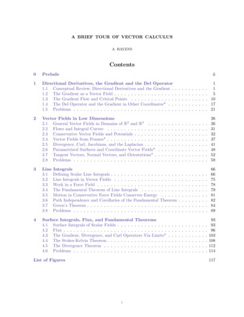
11/14/19Multivariate Calculus: Vector CalculusHavensand D is an n-dimensional subspace of Rn , then the level sets have dimension at most n 1 (this isthe difference of the dimension of the domain and the dimension of the codomain). For example, adifferentiable two-variable function has level sets which are generally curves, while a differentiablethree variable function has level sets which are generally surfaces.Example 1.1. Let f (r) r · r. The value of f at a point r Rn is the square of the distanceof r from the origin 0 Rn . The level sets are spheres; in 2D the level sets are the “1-sphere”S1 , i.e., the circle, while in R3 they are the familiar “2-sphere” S2 , which is the surface of whatnon-mathematicians think of when they hear the word sphere. A quick calculation shows that thegradient of f is 2r, which is a radial vector field, pointing away from the level sets outwards (towardsmore distant level sets). This is depicted for 2 and 3 dimensions below in figure (3).Figure 3. The level sets and gradients of the square distance function f (r) r · rin 2 and 3 dimensions.Note that the gradient in the above examples is in a sense perpendicular to the level sets themselves (namely, it is perpendicular to the tangent spaces at any point of a level set). It turns outthis is not merely because the level sets of the previous example were circles and spheres, while thegradients in the previous examples were radial. More generally, we should expect the directionalderivative to vanish along directions tangent to level sets, since the value of the function doesn’tchange along a level set. Another intuition is that since the gradient tells us how to move away fromP to most steeply ascend through values of f , we expect that the gradient should “point as muchas possible away from level sets”. One can show explicitly using the chain rule that in fact, thegradient is always orthogonal to the level sets (in the sense that it is perpendicular to any tangentvector):Proposition 1.2. For a given level set S f 1 (k) of a differentiable function f : D R, andany point P S, let r0 be the position of P andTP S {v Rn : v γ̇(t0 ) for γ : I S a curve in S with γ(t0 ) r0 }be the tangent vector space to S at P , i.e. the set of tangent vectors at the point P to curves in Sthrough P . Then f (P ) · v 0 for all v TP S .Thus the gradient of f along a level set S is a normal vector field to S. We’ll explore tangentand normal vectors in greater detail below in section 2.4.6

11/14/19Multivariate Calculus: Vector CalculusHavensExample 1.2. The following example goes through the solution to Exercise 3.3 from the notes onpartial derivatives.While exploring an exoplanet (alone and un-armed–what were you thinking‽) you’ve slid partway down a strangely smooth, deep hole. The alien terrain you are on is modeled locally (in aneighborhood around you spanning several dozen square kilometers) by the height functionz f (x, y) ln»16x2 9y 2 ,where the height z is given in kilometers. Let ı̂ point eastward and ̂ point northward. Your currentposition is one eighth kilometers east, and one sixth kilometers south, relative to the origin of the(x, y) coordinate system given. You want to climb out of this strange crater to get away from therumbling in the darkness below you.Figure 4. The graph of the surface z lnp16x2 9y 2 .(a) Find your current height relative to the z 0 plane.(b) Show that the level curves z k for constants k are ellipses, and explicitly determine thesemi-major and semi-minor axis lengths in terms of the level constant k.(c) In what direction(s) should you initially travel if you wish to stay at the current altitude?(d) What happens if you travel in the direction of the vector (1/8)ı̂ (1/6) ̂? Should you trythis?(e) In what direction should you travel if you wish to climb up (and hopefully out) as quicklyas possible? Justify your choice mathematically.(f) For each of the directions described in parts (c), (d), and (e), explicitly calculate the rateof change of your altitude along those directions.Solutions:p(a) From z f (x, y) ln 16x2 9y 2 , your current height relative to the plane z 0 is z f (1/8, 1/6) ln16Ä ä218Ä 9 16ä2 ln»1664 936 12 ln 2 0.3466 .Thus you are about 35 meters (a bit shy of 115 feet) below the plane z 0.7

11/14/19Multivariate Calculus: Vector Calculus(b) Rewrite f as f (x, y) 12Havensln(16x2 9y 2 ). Then if z f (x, y) k for a constant k, we have1ln(16x2 9y 2 ) 2k ln(16x2 9y 2 )2 e2k 16x2 9y 2k x2y2 1 2k 2k e /16 e /9Çxek /4å2Ç yek /3å2Thus the level curves are ellipses with semi-major axis length 13 ek and semi-minor axislength 14 ek . See figure 5 for a visualization of the contours.(c) To stay at the current altitude, you should initially choose a direction tangent to the levelcurve through your position. To calculate such directions, you can exploit that the gradientat a position r is perpendicular to the level curve through r. The gradient of f is f (x, y) Å9y16xı̂ ̂ ,16x2 9y 216x2 9y 2ãÅãwhich gives a gradient at the starting position of (1/8, 1/6) as f (1/8, 1/6) 4ı̂ 3 ̂ .The perpendicular directions in which you could initially head to stay at the current altitudeare 3ı̂ 4 ̂ .(d) You can compute the directional derivative in the direction of the vector (1/8)ı̂ (1/6) ̂to see what is happening to your altitude. Letû (1/8)ı̂ (1/6) ̂34 ı̂ ̂ .k (1/8)ı̂ (1/6) ̂k55ThenDû f (1/8, 1/6) f (1/8, 1/6) · ûãÅ43 (4ı̂ 3 ̂) · ı̂ ̂55 12 1224 .55Thus, if you head in this direction, you are descending at an initial rate of nearly 5meters downward per meter forward. Indeed noting that this vector is in the exact oppositedirection as your initial position, it heads straight for the origin, which is where the hole isindefinitely deep. So you should not head this way if you hope to live very long.(e) To climb out as quickly as possible, assuming you can maintain stamina, you should seekthe route of steepest ascent, which is a route along the gradient direction. Starting from(1/8, 1/6), you should then initially travel in the direction of f (1/8, 1/6)/k f (1/8, 1/6)k 435 ı̂ 5 ̂. Note that this direction is not the radial direction as one might initially suspect; thisdiscrepancy of directions is sensible given that the level curves are not circles, but ellipses.In fact, we can calculate the cosine angle between the direction of steepest ascent and theradial direction easily: just dot the corresponding unit vectors:ûr (1/8, 1/6) · f (1/8, 1/6)3443 ı̂ ̂ ·ı̂ ̂ 24/25 ,k f (1/8, 1/6)k5555Åã Åãwhence these directions make an angle of arccos(24/25) 0.2838 radians, or 16.26 .8

11/14/19Multivariate Calculus: Vector CalculusHavenspFigure 5. A color map of the altitude z ln 16x2 9y 2 , showing also the elliptical contours for z, and the gradient vector field (with vectors scaled down forclarity).(f) For (c) the rate of change in the altitude is 0, as is easily verified by computing a directionalderivative. It better be zero of course– if you wish to remain at the current altitude, thenheight function should not change initially in the direction chosen. For part (d) the rateof change was computed above as 24/5. For part (e), the rate of change in the gradientdirection is k f (1/8, 1/6)k k4ı̂ 3 ̂k 5. Note these rates represent (kilo)meters ofincline or decline relative to a horizontal (kilo)meter displacement along a vector û S1 R2 .In the preceding example, we used that the gradient of a bivariate function determines thedirection of steepest ascent on the graph surface and that the gradient is perpendicular to levelcurves. Pushing this idea further, we can use that the gradient is normal to level sets S to determinean equation of the affine tangent space to a hypersurface S D Rn given as the level set of somefunction f : D R. Without loss of generality, we can assume such a hypersurface is given as thelevel zero set of an appropriate function. First, we define the affine tangent space:Definition. Let S be a hypersurface given as the zero set f 1 (0) of a

comfort with college level algebra, analytic geometry and trigonometry, calculus knowledge including exposure to multivariable functions, partial derivatives and multiple integrals, the material of my notes on Vector Algebra, and the Equations of Lines and Planes in . 2 on the graph of a function along planes of constant y and xrespectively.