Transcription
THE SECRET BOOKOFFRC LABVIEWGeoff NunesTeam 1391Westtown SchoolVersion 0.19 October 2013
Geoff Nunes, 2013
iiContentsIntroduction. 1Chapter 1 — Elements of LabVIEW Programming . 2The Elements . 2LabVIEW Programs. 3Back to the List . 5Variables . 5Expressions and Assignments. 7Conditionals . 10Flow Control . 12Subroutines . 18Clusters . 20Graphing More. 21Problems . 22Chapter 2 – State Machines . 25Planning . 25Programming. 27Adding a Timeout . 33Delays . 35Problems . 38Chapter 3 — Introduction to the cRIO . 40LabVIEW Projects . 41Running Programs on the cRIO . 44Chapter 4 — The Robot Framework . 49Robot Main . 49Begin . 51Periodic Tasks. 52Robot Global Data . 53Teleop . 55(Very) Basic Teleop Code . 55Waiting Without Hanging. 56Avoiding a Death Spiral. 58Teleop Strategy . 60Autonomous. 60
iiiThe Most Important Part of This Section . 60How Autonomous Works . 60The Autonomous Code . 61Disabled, Finish, and Test. 63Building, Running, and Debugging . 64The Driver Station. 67Developing Code Without a Robot. 71Chapter 5 — Input and Output. 73The Interface Sheet . 73Joysticks. 74Motors . 74Robot Drives . 75Drive Delays . 75Digital Input and Output . 76Input . 76Output . 77Relays. 77Encoders. 77Analog Input . 80Pneumatics . 81The Compressor . 81Valves . 82Doubles . 83Singles. 83Servo Motors. 84Chapter 6 — PID Control . 85PID Math. 85Motor Math . 87Driving Simulator . 89Turret Simulator. 93Final PID Thoughts. 94Problems . 94Chapter 7 — Image Processing. 96Doing it on the laptop . 96
ivLoading an image. 96How LabVIEW stores images . 97Image types . 99Getting images . 100Getting good images . 101Choosing your colors . 103Finding the BLOBS . 105Camera Optics. 107Finding the target distance . 108Advanced Stuff . 112Chapter 8 — The Dashboard . 114Basic Dashboard Communication. 114The Dashboard Project. 116Under the Hood (or Behind the Dashboard) . 116Loop 1: Simple Data Communication . 117Loop 2: Image Acquisition . 118Loop 3: Autobound Variables. 119Loop 4: The Network Table Tree . 120Loop 5: Kinect Data and Display. 120Loop 7: Window Size and Position . 121Loop 6: A Whole Lotta Stuff . 121Dashboard Strategies . 127Building Your Dashboard . 127
1IntroductionThe motivation for this book comes from my own experience as an FRC mentor. At work Iam (or at least pretend to be) a generally competent LabVIEW programmer. I’ve done somepretty cool stuff, like programming a robotic microscope that can automatically inspect a bigsheet of glass: big enough to hold eight 32” flat panel TV screens. My first encounter withFRC LabVIEW, however, transformed me into a gibbering idiot. There is an elaborate, butmysterious, framework that runs the robot, and the main source of documentation seems tobe the forum archives at Chief Delphi. The experts who regularly contribute there are great,but as I was madly trying to learn, and at the same time teach our team members, I foundmyself constantly wishing for a book that explained everything in one place. Hopefully, thisis that book.The intention here is that you can read the entire book, or only the parts that interest you.You can use it as a classroom text, or as a reference manual. Chapter 1 covers the basic principles of programming in LabVIEW. It is written under the assumption that you have already done at least some programming in a “traditional”, text-based language, although ifyou haven’t you should still be fine. Chapter 2 covers state machines, which are essential forprogramming robots. Chapter 3 introduces LabVIEW projects, which is how you manage allthe code for your robot, and Chapter 4 covers the specific project that is the FRC RobotFramework. This chapter is where most of the secrets are revealed. Chapter 5 covers the various input and output devices, such as motors and sensors, you can attach to and control withyour robot. Chapters 6 and 7 cover PID control and image processing. They contain muchthat can be done without a robot, and so can be covered in the pre-season, in spite of appearing later in the book. Finally Chapter 8 covers the Dashboard, which is simple to use, butcomplicated to understand.This book includes, as a companion volume, a zip file of images for use with Chapter 7.Although this book contains many example programs, you won’t find a companion zip filefor them. It takes practice to learn how to write compact, readable LabVIEW code, practiceyou will get by diagramming the examples yourself.As you read this book and compare it to the actual software, please be aware that we are aiming at a moving target. A new version of the FRC robot framework is issued every year, andevery year there are improvements and enhancements. You can pretty much be guaranteedthat if you are building a robot in year , this book was updated against a version of theframework from the year 1. (Or 2. Or worse.) Be flexible.Finally, a note of thanks to both Worcester Polytechnic Institute and National Instruments.The FRC robot framework is a product of the robotics program at WPI, and is a large, complex, and amazingly robust piece of software. Without it, FRC would be way more work andway less fun. Equally amazing is the support that NI provides to FRC, as is the amount oftime an effort their staff contribute on Chief Delphi and at competitions. I owe a particulardebt to Greg McKaskle, whose white paper on vision targeting for the 2012 competition inspired much of Chapter 7.
2Chapter 1 — Elements of LabVIEW ProgrammingThis chapter is designed to get you up and running with LabVIEW as quickly as possible. Itis probably a terrible way to actually learn LabVIEW. For that, I would recommend “LabVIEW for Everyone” by Jeffrey Travis and Jim Kring (Prentiss Hall, New York, 2006). It isa very complete book. It also thick enough to stun an ox.You should read this chapter with your computer on and LabVIEW open. And you shouldactually program all the examples for yourself. LabVIEW is an “experimental” programming language in the sense that you will learn by doing experiments to see what happens. Ifyou take a “reading only” approach, you will never really learn, and that will be very frustrating.The ElementsAll programming languages share a set of common elements. If you have written programsin a text-based language (e.g., C and friends, Java, FORTRAN, BASIC, Python ), then youwill be at least vaguely familiar with these elements. I’ll give them a quick listing, and thenrevisit each one to show how it appears in LabVIEW. If you know all this already, then justjump ahead to the LabVIEW part.1. Variables These are objects in which you can store data. They might hold a single number, or an array of numbers, or a string of text. Boolean variables can be either True or False.2. Expressions These are the operations that manipulate the values stored in variables, as inA B.3. Assignments This is how you get values into variables. For example, you might assign avariable to have constant value, as in PI 3.1415. Or you might use an expression to give avariable a value based on other variables, as in C A B.4. Conditionals Also called branching statements. The simplest conditional allows one pieceof code to execute if an expression evaluates to True, and a different piece to execute if theexpression evaluates to False.5. Flow Control This is the term generally applied to sections of code that repeat for a setnumber of times, or repeat until some condition is true. Strictly speaking, conditionals alsocontrol the flow of a program, so the distinction between them and flow control elements is abit arbitrary.6. Subroutines These are any pieces of code that can be packaged and used in some otherpiece of code. They go by lots of other names: function, procedure, or subprogram.We’ll stop the list here, and point out that you are not even a single page into this book andhave already encountered its first lie. (Note the clever implication that there will be more liesto come.) I said at the start that all programming languages share a common set of elements,but that is not true. In a text-based program, an assignment, or a print command, or a command to write to a file, all go by the generic term statement. LabVIEW doesn’t have statements. It is an entirely different kind of beast.
3LabVIEW ProgramsBefore we revisit the list of elements, it is necessary to spend a moment on the structure ofLabVIEW (LV for short) programs. In a text-based language, a (simple) program is just asingle object: a text file. In LV, a program is two objects: a front panel which handles inputs and shows you the results, and a block diagram which contains the actual code. If youwant, you can think of the front panel as the body and controls of a car: it’s got the fancypaint job, the headlights, turn signals, steering wheel, and pedals. The block diagram is theengine that makes it go.When you start LabVIEW (do it now) you get a window that looks something like Fig. 1.1.If it doesn’t say “FRC” somewhere on this screen, you haven’t installed everything that youneed, and won’t be able to follow much of this book.FIGURE 1.1 The LabVIEW Getting Started window.Click on “Blank VI”, and you will get a pair of windows, like Fig 1.2. The windows areconveniently labeled so you can see right away which one is the front panel and which one isthe diagram. You will need to toggle back and forth between these two windows a lot. Theeasiest/fastest way to make this swap is with the ctrl-E key combination.FIGURE 1.2 A new VI (LabVIEW program) showing the front panel(foreground) and block diagram (background).
4To make this more concrete, Fig. 1.3 shows the front panel of a simple program (which hasbeen run once to draw the data on the graph), and Fig. 1.4 shows the diagram that makes itwork.In LV, a program is officially called a VI, which is short for Virtual Instrument. I will usethe terms “VI” and “program” interchangeably. Although the program in Figs. 1.3 and 1.4doesn’t do much, there is a lot of new “LabVIEW-ey” stuff going on. I promise that you willsoon understand it all. But in order to do that, we need to get back to the list.FIGURE 1.3 The front panel of a LabVIEW program. This program has been run. Otherwise, the graph would be blank.FIGURE 1.4 The block diagram of the program in Fig. 1.3.
5Back to the ListVariablesJust as the programs have two parts, variables in LV have two parts: the thing that appearson the front panel, and the corresponding terminal on the diagram. They also come in two“flavors”, depending on whether you read from them, or write to them. In Figs. 1.3 and 1.4,the objects labeled “No. of points”, “x start”, and “x end” are all controls. The programreads from them. The object labeled “XY Graph” is an indicator. The program writes to it.This division is very strict: variables are either controls or indicators. The program eitherreads from them, or writes to them, but not both. (There is a way around this using local variables. We’ll get to them later.)One of the cool features of LabVIEW is that variables can have names thatwould be illegal in any other language. They can have spaces and symbols andpunctuation if you want. You can even give two different variables the samename! LabVIEW will always know which one is which, although you will not.Don’t do this.The most common method for adding a variable to your program is from the front panel.Open a blank VI, and right-click on the front panel. You should get a pop-up menu thatlooks something like the left-hand side of Fig. 1.5. To get the right-hand side of the figure, Islid the mouse over the upper left square, and the Numeric sub-menu popped open. Movethe mouse over each item, and you get its name shown at the top. Everything here is either acontrol or an indicator. In theFIGURE 1.5 The Controls Palette for placing objects on the front panel.
6upper left is a numeric control. To its right is a numeric indicator. They are not really different, except values are read from one and written to the other. In the second row, the leftmost object is a vertical fill slide (an indicator) and next to it is a vertical pointer slide (a control). There is no significant difference between the slider control and the text box control!In one case, you type the value you want the variable to have. In the other you move theslider until it has the value you want. The slider defaults to a zero to ten range when youdrop it on the front panel, but you can double click on the starting and ending values andchange them to anything you like. Similarly, there is no real difference between the indicators except how the value is displayed. In fact, both can have a digital display that you typeinto or read from, making the slider part pure eye candy.One of the best designed and most powerful tools in LV is the right click,which brings up the context menu. As the name implies, the contents of thismenu depends on the context in which you right-clicked. You should get inthe habit of—as an experiment—right-clicking on things, and examining thelist of options that is presented. If I tell you to do something in this book, but Idon’t tell you how, you can bet that it involves a right-click. I’ll highlight a few key rightclicks as we go along, but there are far too many options to cover in a skinny volume like thisone. Explore, explore!If you haven’t fixed it yet, the controls panel you get by right-clicking on thefront panel looks nothing like Fig. 1.5. Probably the Express controls are thedefault. They are very limited, and you should fix yours to look like mine. Notethe little thing that looks like a push-pin in the upper left of the palette. It is apush pin. Click on it and the palette is “pinned” to the screen. When you dothat, a Customize button will appear, which will allow you to put the Modern palette at thetop, and also control other aspects of how the palette looks. (I am really particular about mywork environment. Time is short, and there is a lot to do. I insist on customizing the LV environment to make my work as efficient as possible. You should too.)In addition to controls and indicators, there is a third variable form, the constant. Constantsare controls that have a fixed value. They appear only on the diagram, as their value cannotbe changed by the operation of the program.In all cases (control, indicator, and constant), these objects also have a specific representation. You are very unlikely to use anything other than the big three: double precision real,32-bit integer, and unsigned 32-bit integer. Once you have created a control, for example,you can right-click on it to change its representation. If you don’t know the difference between a real and an integer in the context of computer programming, this book is not theplace to learn it!Variables can hold just a single value, or they can be arrays of values. These arrays can beone-dimensional, two-dimensional, or n-dimensional. There are also more complicated objects that are the equivalent of structures in C. In LV, these are called clusters in which several different kinds of objects (e.g. a real number, a Boolean, and an array of integers) can allbe bundled together in a single object. You will find that clusters are common in FRC programming.
7Expressions and AssignmentsTime to learn by doing! We’ll write a program that executes the statement “C A B”, except that it won’t be something you recognize as a statement (i.e. as a line of code). Create anew, blank VI. On the front panel, place two Numeric Controls named A and B, and a Numeric Indicator named C. Your front panel should look something like Fig. 1.6.Flip over to viewing the diagram, you will have something that looks nothing like Fig. 1.7.To begin with, unless you have already fixed this, your terminals are not sleek and svelte likemine, but big, blocky, and awkward. Also, your terminals are probably randomly scatteredabout the diagram, and not neatly arranged in anticipation of the connections to be made.You should fix both of these things. To change how terminals appear, go to the Tools menuand select “Options ”. Select the Block Diagram category and un-check “Place front panelterminals as icons”. The new setting will apply to any new objects you create, but won’tchange the objects you’ve already put in your program. You get only one guess as to how tobring up a menu that will let you change how the already placed terminals appear. You willhave to do that for each one.FIGURE 1.6 The front panel of a very simple program.FIGURE 1.7 The block diagram for Fig. 1.6.Right-click on the diagram to bring up the Functions Palette. If it doesn’t look like mine(Fig. 1.8), or like the way you want it to, then pin it and customize it, just as you did with theControls Palette. Find the Numeric sub-palette, select the Add function, and place it on yourdiagram. I’ve laid out the terminals in a suggestive fashion, and it should be obvious whereit goes.Now we need to connect things up. Hold down the shift key and right-click on the diagram.This brings up the Tools Palette (Fig. 1.9). You need to use the little spool symbol on theleft, so you could select it. But it is much better to select the Multipurpose Tool at the top,which will automatically give you what you need, depending on where you move the mouse.In Fig. 1.9, the Multipurpose Tool has been selected.It takes some getting used to the spool tool. When drawing a wire that has toturn corners (as in Fig. 1.10 below), you can click to set the location of the corner. You will notice that the tool is always trying to draw a vertical line segment, or a horizontal one. You can force it to switch from one to the other
8(while drawing a wire) by hitting the space bar. Also, go to the Tools menu and select “Options ”. Select the Block Diagram category and, under the Wiring sub-category, un-check“Enable automatic wire routing”. But leave “Enable auto routing” checked. (Trust me.They are different!)FIGURE 1.8 The Functions Palette.FIGURE 1.9 The Tools Palette.Now, with the Multipurpose Tool selected, if you hover the mouse over the little black triangle on the A terminal, the cursor should change to a spool. Click to start the wire, and connect it to the B terminal. This is wrong, and LabVIEW will tell you in two ways. The wire isdrawn as a dashed line with a big red X, indicating that it is a broken wire. If you look in theupper left of your diagram (or front panel), you will see that you have “broken arrow” syndrome. A LabVIEW program with a broken arrow will not run. You can clear broken wiresby selecting and deleting them, or you can use the ctrl-B key combination to delete all thebroken wires in your program at once. (Use ctrl-B with caution. Sometimes a simple problem will cause all of a complex diagram to appear broken. Fixing that simple problem willbe much less work than re-drawing the entire diagram.)So, clear the broken wire, and wire the diagram to match Fig. 1.10. From the front panel youcan type values into A and B, and hit the (un-broken) white arrow in the upper left to run theprogram and have the result of the addition assigned to C.What did you not do? In languages like Java and C, you need to compile and link your program before you can run it. LabVIEW does all that automatically and more or less instantly.If you have the white arrow, your program is ready to run. (To be fair, that is only true forprograms that run on your computer. You will need to compile your robot programs, but thatdoesn’t happen until the next chapter.)
9FIGURE 1.10 Our simple program, all “wired up.”.The multipurpose tool can be a bit tricky if you are using it to drag wires aroundon your diagram. I like a neat, easy to read diagram, so I select and drag thewires to where I want them. It is really, really easy to click on a wire, only tofind that the move tool (a pointer arrow) changed to a wiring spool just as youclicked, so now you are adding a new wire to your wire instead of moving it.Hit the Escape key or right-click to get out of situations like this.LabVIEW contains several automatic tools for neatening up your diagram. I amnever quite happy with the results, so never use them. You may have a differentopinion.As I promised, there is no explicit assignment statement. The wires in Fig. 1.10 are LabVIEW’s equivalent of assignment statements. But don’t think of them like that. Think ofthem as wires. Data flows
Chapter 1 — Elements of LabVIEW Programming This chapter is designed to get you up and running with LabVIEW as quickly as possible. It is probably a terrible way to actually learn LabVIEW. For that, I would recommend “Lab-VIEW for Everyone” by Jeffrey Travis and Jim Kring (P r