WIXLIB

IICHAPTER 1INTRODUCTION1.1What is Data Mining?Data mining is a technique to discover patterns and trends in data and to create a statisticalmodel of that data. It is particularly useful for large, high dimensional data sets that aretoo unwieldy for traditional statistical analysis. Unsupervised learning refers to the task ofdescribing patterns in the data while supervised learning refers to the task of building pre dictive models. If the quantity to be predicted in supervised learning is a numerical value,then regression analysis is performed. If, however, the quantity to be predicted can onlytake on a finite number of values, then classification is performed. Binary classification isundertaken when there are only two possible values for the output quantity.An important binary classifier is the Support Vector Machine classifier (Boser, Guyon,and Vapnik 1992) (Vapnik 1996), which classifies data based on its relative location to aseparating hyperplane. In order to find this separating hyperplane, a quadratic programwith inequality constraints is solved to obtain the equation of the separating hyperplane.However, due to the nonlinearity of the objective function, obtaining the solution can bedifficult. Kecman and Arthanari (2001) attempted to remedy this problem by replacing thequadratic term in the objecfive function of the Support Vector Machine classifier (SVM) bya linear term. Fung and Mangasarian (2001) also reformulated SVM to decrease solutiontime and created the Proximal Support Vector Machine classifier (PSVM). Their classifierhas a purely quadratic objective function. In addition, they replaced the inequality con straints with equality constraints. The Karush Kuhn Tucker conditions can then be used toobtain the solution from a system of linear equations.The Proximal Support Vector Machine classifier, while quick to solve, magnifies theimportance of points far from the hyperplane. In order to remedy this, we propose the

12Linearized Proximal Support Vector Machine classifier. This is a reformulation of PSVManalogous to Kecman and Arthanari's reformulation of SVM.All Support Vector Machine classifiers try to minimize the number of potential errorsthe classifier will make by minimizing a sum of distances from a hyperplane. However,the actual task of classification does not place any importance on the distance from theclassifying hyperplane and is only concerned with the relative location of the point to beclassified. In order to model this more closely, we propose the Integer Support VectorMachine Classifier (ISVM). ISVM uses binary error indicator variables to minimize thenumber of potential errors the classifier can make.The structure of this document is as follows: Chapter 2 gives the formulation for Lin earized PSVM, discusses results for a simple two dimensional data set, and gives resultsfor eleven data sets from the UCI Machine Learning Repository (Blake and Merz 1998).Chapter 3 presents similar information for a reformulation of SVM as an integer program.Chapter 4 presents an apphcation of linear classifiers to collusion detection in online gam bling. The final chapter. Chapter 5, summarizes the previous chapters and discusses futureresearch directions.Data mining is highly application driven, meaning the solution technique is driven bynot only the data, but the question that the owners of the data want answered. Data setscome from diverse fields, including biology and health care, computer science (image pro cessing), business and marketing, and physics. Applications from biology and health careinclude predicting the recurrence of cancer in patients (Mangasarian, Street, and Wolberg1995), predicting which new chemical compounds are likely to result in new drugs (Srinivasan and King 1999), and predicting which patients are likely to develop diabetes (Smith,Everhart, Dickson, Knowier, and Johannes 1988). Applications from computer science in clude image classification (Schweitzer 1997), spam filtering (Androutsopoulos, Koutsias,Chandrinos, and Spyropoulos 2000), and detecting intrusion into computer systems (Han,Lu, Lu, Bo, and Yong 2002). Business and marketing uses data mining for targeting ad vertisements to customers to maximize their effectiveness (Ha, Bae, and Park 2002). Data

13mining is also used to discover which products people are likely to buy together to improveproduct placement in stores (Hamuro, Katoh, Matsuda, and Yada 1998). Finally, physicsuses data mining to process the massive amounts of data collected in particle collisionexperiments (Conway and Loomis 1995) and to examine the large amounts of data pro duced by N-body astrophysics simulations (Pfitzner, Salmon, and Sterling 1997). With thediversity of fields, the terminology used by practitioners can vary widely. The set of mea sured variables is known as the inputs, features, predictors or independent variables.Those variables that are influenced by the measured variables are known as the outputs,responses or dependent variables. The output variables may not always be included inthe data set.Input variables can be one of three types: quantitative, qualitative (or categorical),and ordered categorical. The values of quantitative variables can be compared and ametric is defined over the set of possible values. A qualitative or categorical variable canonly take on values from a finite set and these values cannot typically be compared, i.e.{red, green, blue). The values of an ordered categorical variable can also only take on afinite number of values, but they can be compared. Unlike quantitative variables however,no metric is defined over the set of possible values. An example of an ordered categoricalvariable is one that can take on the values {small, medium, large).Following the notation in Hastie et al (2001), X is an input variable or feature. If X is avector, Xj is the j"' component of X. Quantitative outputs are denoted as Y and qualitativeoutput are denoted as G. Xi is thetheobservation of input X and Xij is theobservation ofcomponent of input X. A series of N observations of the input vector X is denotedX — ( 1) 2 : 5 AT)*The data mining process consists of five steps: acquiring the data, cleaning the data,training the model, model validation, and model use. The first step, data acquisition, canbe the most difficult step from a practical viewpoint. Unless the data set already exists,the collection system must be designed and tested. In addition, the storage system mustbe designed and implemented. Often data mining is not undertaken unless the data already

14exists and is easily accessible.The second step prepares the data for mining. There are several tasks that must takeplace here. First of all, the data set may be missing values and a procedure for processingthose values must be determined. Options include excluding those data points with missingvalues and excluding that particular feature from the feature set to be mined. In the case ofnumerical data, a particular value (for example 0) may be assigned if appropriate. In thecase of categorical data, the missing values may be treated as a separate category. Addi tionally, any aggregate features should be calculated. Aggregate features are those that arecomputed from other features such as averages, variances and even time information suchas day of week, day of year, or month.Training the model involves choosing an appropriate algorithm and applying it to thetraining data set to build a model. Algorithm choice is driven by the specifics of the problemto be solved as well as the data itself. To validate the model after it is built, its performanceis evaluated on the test data set. The test set should not contain any data previously usedin training the model. Typically, one large data set is spht into two pieces, not necessarilyof equal size. One piece is used for training the model and the remaining piece is used fortesting. Once a model is created with satisfactory performance, the model is used.One issue in creating the training and test data sets is determining how much data touse in each set. Physical limitations of computing environments, i.e. disk space, RAM andCPU speed, may severely limit the amount of data used. One strategy has been proposedby Yakowitz and Mai (1995) in the machine learning literature. Their strategy was origi nally devised for the task in sequential design of determining the minimum of an unknownmeandering function based on a set of measurements with noise. In this sequential designproblem, an experimenter obtains a number of these noisy measurements, which can betaken at any point without penalty for poor choices. The experiment will be terminated atsome period in time and the experimenter neither controls this point nor has knowledgeof when it is. At the end of the experiment, the experimenter must specify the point theyconsider to be the best on the basis of experimentation. Yakowitz and Mai propose an off

15line learning method that seeks the best trade-off between acquiring new test points andretesting previously selected points to maximize performance. This method could be usedto determine experimentally when to add new points to a test or training set.1.2 Methods Used in Data MiningData mining methods can be split into two groups according to the task they perform.Unsupervised learning methods are given a set of inputs and try to learn properties aboutthe joint probability distribution function of the features. Supervised learning methods aregiven a set of inputs and attempt to predict the output variables.1.2.1Unsupervised Learning MethodsThe data for an unsupervised learning task consists of N observations {xi,x2,. , xn) ofa p-dimensional random variable, X, and try to learn properties of the joint probabilitydistribution function /(X) in the absence of any error information (i.e. the true outputvariable is not available). For low dimensional data sets (3 or fewer dimensions), techniquesfrom statistics can be used to estimate /(X). However, these techniques are not applicablefor higher dimensional data sets (p 3) because as the number of dimensions increases,the density of sample points decreases and the estimates become less reliable. In this case,most of the methods use descriptive statistics, i.e. they try to determine characteristics ofthose X's where /(X) is large. This can be done by creating new features that are functionsof old features as in Principal Components, Self-Organizing Maps and MultidimensionalScaling. Or, as in Cluster Analysis, we can try to directly find regions where /(X) is large.Principal Components, Principal Curves, Self-Organizing Maps, and Multidimen sional Scaling attempt to reduce the dimensionality of the data set by determining whetherthe variables are functions of a smaller set of "latent" variables. Principal Components andPrincipal Curves (Hastie, Tibshirani, and Friedman 2001b) find series of approximations tothe data. Principal components finds a series of linear approximations to the data by least

16squares approximation. These Hnear approximations are orthogonal projections of the dataonto a line or plane. The first linear approximation in the series has the highest variance andsubsequent approximations decrease in variance. Principal Curves is the generalization ofPrincipal Components to non-linear projections. Self-Organizing Maps (Hastie, Tibshirani,and Friedman 2001c) overlay a grid of integer points (called "prototypes") over the data setand bends this grid space until the prototypes approximate the data as well as possible. Thisprocedure does not preserve relative distances between points, which in some applicationsis desirable. Multidimensional Scaling (Hastie, Tibshirani, and Friedman 200Id) attemptsto remedy this by trying to preserve the distances between the data while finding a lowerdimensional approximation of the data.Cluster Analysis (Hastie, Tibshirani, and Friedman 2001e) assumes that the data can berepresented as a mixture of simpler densities or clusters. Each individual density is assumedto represent a class in the data. In i -means clustering (Hastie, Tibshirani, and Friedman200 le), K cluster centers are chosen, one for each class. Each data point is assigned tothe class corresponding to the closest cluster center. The positions of the cluster centersare moved around in an iterative fashion until the points within a cluster are closer to eachother than they are to points outside the cluster. Finally for binary-valued data. AssociativeRules (Hastie, Tibshirani, and Friedman 2001f) attempt to discover joint conjunctive rules,i.e. sets of variable values, that describe regions of high density.Model validation for unsupervised learning tasks can be somewhat problematic as noerror informaUon is contained within the data set. The model validation process must thenrely on heuristics to evaluate model quality.1.2.2 Supervised LearningSupervised learning is somewhat easier than unsupervised learning since an outcome foreach observation X (xi, X2,., xat), where Xi is a random p-vector, is included inthe data set. In the case of a numerical outcome, Y, regression, which seeks to predict a

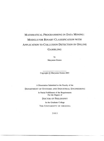
17numerical value, is used. For a categorical outcome, G , classification is attempted.Regression tries to make a good prediction, Y, of the quantitative output given a valueof the input X. Least squares regression is a well-known example of this. Linear leastsquares (Hastie, Tibshirani, and Friedman 200 Ig) models the output, Y, as a linear com bination of the components of the input p-vector X (Xi, X2,. Xp). The task is to findthe coefficients of X. This is done by minimizing the residual sum of squaresRSS(/3) (y-/3Xf (y - X).Other methods that fall into the regression category include basis expansions (splines,wavelets, etc.), kernel methods, and neural networks. Basis expansions (Hastie, Tibshi rani, and Friedman 200Ih) uses a set of m functions, hm{X) : JR'' 3R, to transformthe input variables into new variables. The model of the outputs is then a linear combina tion of the transformed variables. Any complete set of basis functions can be used as thetransformations including splines and wavelet transformations. Kernel methods (Hastie,Tibshirani, and Friedman 200 li) fit a model, which can be linear or polynomial for exam ple, to each point, Xo, using its neighbors, i.e. points "close" to it. The kernel Kx{Xo, Xi) isa function that determines the neighborhood of Xo by setting weights on the rest of the datapoints Xj. The parameter A sets the width of the kernel.Neural networks (Hastie, Tibshirani, and Friedman 200Ij) were developed separatelyin the statistics and artificial intelligence fields. A neural network consists of two stages.First, new variables that are Hnear combinations of the inputs are created. The output ismodeled as a non-linear function of the inputs. A simple neural network is shown in Figure1.1. The variables in the hidden layer, Z, tire modeled as a function of linear combinationsof the inputs XZ o (aom , m 1,., M,where a ( v ) is the activation function. Traditionally, the sigmoid function is used. The

18output Y is then modeled as a function of a linear combination of the hidden variablesY fiX) :g(/3o ''Z).Output LayerHidden LayerInput LayerFIGURE 1.1. A graphical depiction of a neural network.Classification tries to determine the class of a particular input X . Support vector ma chines, neural networks, classification trees, and fc-Nearest-Neighbor classifiers are all ex amples of classification algorithms. Support vector machines (Hastie, Tibshirani, andFriedman 2001k), as explained in more detail in Section 1.4, use constrained optimiza tion to find hyperplanes separating classes of data. These hyperplanes define regionsof space for the classes. A point is classified according to the region of space it fallsinto. Neural networks (see above) may also be used for classification. Here, the neuralnetwork is generalized to the multi-output case. Each of the outputs represents a par ticular class and is constrained to lie in the interval [0,1]. There is one output function

19QkWok -'r P'k )i k 1,. J K for each of the K outputs that is a function of a separatelinear combination of the hidden variables. If the soflmax function,gTfc9k { T ) where— ok /3'[Z, k 1,., K, is used, the numerical value of the k output ispositive and the values of the output functions sum to 1 (Hastie, Tibshirani, and Friedman200Ij). The value of the output can be interpreted as the probability that a point is inclass k. Classification trees (Hastie, Tibshirani, and Friedman 20011) typically split thefeature space recursively into regions. Observations in a node are classified according tothe majority class in that node. K-Nearest-Neighbor classifiers (Hastie, Tibshirani, andFriedman 2001m) classify a point based on the class of its nearest neighbors.Model evaluation is somewhat easier for supervised learning tasks as the model pre diction can be compared to the actual outcome. For regression, a loss function is defined,which is a function of the difference between the actual outcome Y and the predicted out come f{X). Typically, squared error or absolute error is used( y — f(X)]L{YJ{X)) V y-fix)squared error absolute errorThe test error is the expected value of the loss function and is calculated over an indepen dent test set. According to Tibshirani et al (2000), training error1 i lis generally a bad estimate of test error. This is because training error can be reduced byincreasing model complexity, thus adapting more and more to underlying structure in thedata. However, this underlying structure may be a peculiarity of the training set (e.g. noise)and may not be present in future data. Models that have adapted themselves too closely tothe data are said to have overfit the data. While such a model will have low training error, it

20will not generalize well and its test error will be large. Other methods are used to estimatethe test error for regression tasks.For classifiers, one simple measure of performance is accuracy. Accuracy is the frac tion of correct predictions. However, Provost et al (1998) argue that comparing accuracyfor classifiers may be misleading. They state that accuracy does not account for differencesin misclassification costs among the classes and is also dependent on class distribu

a particular item belongs. An important binary classifier, the Support Vector Machine classifier, uses non-linear optimization to find a hyperplane separating the two classes of data. This classifier has been reformulated as a linear program and as a pure quadratic program. We propose