Transcription
BMI 713: Computational Statistics for Biomedical SciencesAssignment 7Simple Linear RegressionTo study the relationship between a father’s height and his son’s height, Karl Pearson (1857-1936)collected the data of heights from 1078 father-son pairs.(a). Get the dataset by the following R data(father.son)Then the data frame father.son contains the 1078 observations on 2 variables: fheight (father’sheight in inches, x) and sheight (adult son’s height in inches, y).(b). Draw a scatter plot of son’s height versus father’s height. Does the relationship appear linear?Sol’n. From the scatter plot below, we can see that the son’s height tends to increase as the father’s heightincreases.6065707580 plot(fheight, sheight, xlab "Father's height (in)", ylab "Son's height (in)",xlim c(58,78), ylim c(58,80), bty "l", pch 20)Son's height (in)1.60657075Father's height (in)(c). Fit the simple linear regression of son’s height on father’s height. What are the estimatedregression coefficients, a and b, respectively?Sol’n. Denote the 1078 father-son pairs of observations as (x1, y1), , (xn, yn), where n 1078.We will fit the linear regression model of son’s height y on father’s height x:y α β x e, e N(0, σ 2 )
Fit the linear model by the method of least squares, and the estimated regression coefficients are:nb (xii 1 x )(yi y )n (xi 1i x)2 Cov(x, y)(slope), 0.514Var(x)anda y bx 33.89 (intercept).We can also fit the linear regression model in R by the function lm: m - lm(sheight fheight) summary(m)Call:lm(formula sheight fheight)Residuals:Min1QMedian-8.877151 -1.514415 e Std. Error t value Pr( t )(Intercept) 33.886601.8323518.49 2e-16 ***fheight0.514090.0270519.01 2e-16 ***--Signif. codes: 0 ‘***’ 0.001 ‘**’ 0.01 ‘*’ 0.05 ‘.’ 0.1 ‘ ’ 1Residual standard error: 2.437 on 1076 degrees of freedomMultiple R-squared: 0.2513,Adjusted R-squared: 0.2506F-statistic: 361.2 on 1 and 1076 DF, p-value: 2.2e-16(d). Add the regression line y a bx to the plot in (b).706560Son's height (in)7580Sol’n. abline(lm(sheight fheight), lty 1, lwd 2)606570Father's height (in)75
(e). Calculate Pearson correlation coefficient r between father’s height and son’s height. Perform aproper test to test the null hypothesis ρ 0 , where ρ is the population correlation coefficient. .Sol’n. Pearson correlation coefficient r is defined asnr (xi 1i x )(yi y ) 2 2 (xi x ) (yi y ) i 1i 1nn Cov(x, y)Var(x)Var(y)We can calculate it in R: r - cov(fheight, sheight) / (sd(fheight) * sd(sheight)) r[1] 0.5013383or using cor function in R: cor(fheight, sheight)[1] 0.5013383To test the null hypothesis ρ 0 , we need to first calculate the standard error of r :1 r2 0.026n 2Under the normality assumption and null hypothesis, the t-statisticSE(r) r 0n 2 rSE(r)1 r2follows a t distribution, with n 2 1076 degrees of freedom.For r 0.501 , the test statistic is t 19 , which gives the p-value less than 1e-10. Thus, we rejectthe null hypothesis ρ 0 .t To test the null hypothesis in R: cor.test(fheight, sheight)Pearson's product-moment correlationdata: fheight and sheightt 19.0062, df 1076, p-value 2.2e-16alternative hypothesis: true correlation is not equal to 095 percent confidence interval:0.4552586 0.5447396sample estimates:cor0.5013383(f).What is the 95% confidence interval for the slope coefficient β?Sol’n. To construct the confidence interval, we first need to determine the standard error of bSE(b) 1 n (y ŷ)2n 2 i 1 in (xi 1i x )2Compute it in R: SE.b - sqrt(1/(1078-2) * sum((sheight-fitted(m)) 2) / sum((fheightmean(fheight)) 2)) SE.b[1] 0.02704874
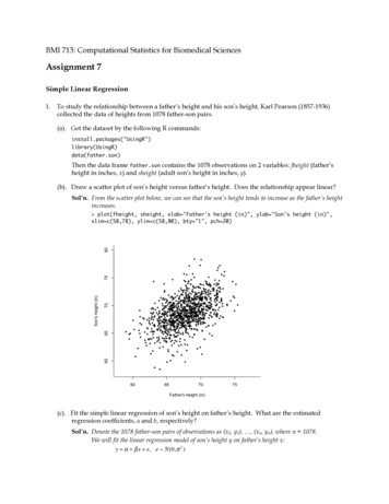
Under the normality assumption, the t-statisticb βt SE(b)follows a t-distribution, with (n-2) degrees of freedom.Then, 95% confidence interval for β is:b t1076, 0.975 SE(b) 0.51409 1.962 0.02705 (0.461, 0.567)(g). Calculate the coefficient determination R 2 . What does the R 2 statistic mean?Sol’n. The coefficient of determination R 2 is calculated asnReg SSR2 Total SS ( ŷ y )2i 1n (y y )i 12iIn R: R.squared - sum((fitted(m) - mean(sheight)) 2) / sum((sheight mean(sheight)) 2) R.squared[1] 0.2513401Here the R 2 statistic is the proportion of the total response variation explained by the explanatoryvariable in the linear regression model.(h). Draw a residual plot. Are the residuals normally distributed with constant variance?Sol’n. The model assumptions of normal distribution and constant variance seem valid based on theresidual plot below.0-5Residuals5Residual Plot646668Fitted values7072
(i).What are the estimated means of son’s height given that his father’s height is 72, 75, 60, and 63inches, respectively?(Notice that sons of tall fathers tended to be tall, but on average not as tall as their fathers.Similarly, sons of short fathers tended to be short, but on average not as short as their fathers.This phenomenon was first described by Sir Francis Galton, as “regression towards mediocrity”,where the term regression came from. The regression effect – phenomenon of regression towardthe mean – appears in any test-retest situation.)Sol’n. The estimated means of son’s heights are 70.9, 72.4, 64.7, 66.3 inches, given that his father’sheight is 72, 75, 60, and 63 inches, respectively.(j).Given a father’s height, we can use simulation method to construct the 100(1-α)% confidenceinterval for the mean of his son’s height. First draw 1000 samples each of size 1078 withreplacement from the 1078 pairs of father-son heights, then from each sample fit a linearregression model by the method of least squares, and compute the estimated mean of son’sheight.What are the mean and standard deviation of these 1000 simulated values?Sort these 1000 estimated means in ascending order. Denote the 25th largest as h25 and the 975thlargest as h975 , which are our estimates of the 0.025 and 0.975 quantiles of the samplingdistribution for the mean of son’s height. Then the 100(1-α)% confidence interval for the meanof the son’s height is ( h25 , h975 ). Compute the 95% confidence interval for the mean of son’sheight if his father is 72 inches tall.Sol’n. Use the following loop to run 1000 simulations in R: n - 1078 h.father - 72 h.son - rep(NA, 1000) for (i in 1:1000) { v - sample(1:n, n, replace TRUE) fheight.sim - fheight[v] sheight.sim - sheight[v] b.sim - cov(fheight.sim, sheight.sim) / var(fheight.sim) a.sim - mean(sheight.sim) - b.sim * mean(fheight.sim) h.son[i] - a.sim h.father * b.sim } mean(h.son) # mean of the 1000 simulated values[1] 70.89778 sd(h.son)# standard deviation of the 1000 simulated values[1] 0.1346589 h.son.sort - sort(h.son) h.son.sort[25]# the estimated 0.025 quantile[1] 70.63136 h.son.sort[975]# the estimated 0.975 quantile[1] 71.1718Thus, the estimated 95% confidence interval for the mean of son’s height is (70.63, 71.17) inches,given that the father’s height is 72 inches.
Contingency Table2.In an investigation of the association between smoking habit and lung cancer, lung cancer patientsand controls were obtained. The patients and controls were matched for age, sex, and community.The data are shown in the table below. (Data from P. Notani and L. D. Sanghvi, “A RetrospectiveStudy of Lung Cancer in Bomby”, Br. J. Cancer 29(6): 477-482, 1974.)SmokersNonsmokersLung Cancer413107Controls318201(a). What is the type of this study in terms of study design?Sol’n. This is a case-control (or retrospective) study.(b). Calculate the odds of lung cancer for smokers, the odds of lung cancer for nonsmokers, and theratio of two odds.Sol’n. The odds of lung cancer for smokers are 413 / 318 1.299, and the odds of lung cancer fornonsmokers are 107 / 201 0.532. The ratio of two odds is 1.299 / 0.532 2.44; that is, the oddsof having lung cancer for smokers are estimated to be 2.44 times as large as the odds of havinglung cancer for nonsmokers.(c).Calculate the 95% confidence interval for the odds ratio.Sol’n. To get a confidence interval for the odds ratio, construct a confidence interval for the log of theodds ratio and take the antilogarithm of the endpoints.The log of the estimated odds ratio is ln(OR̂) ln(2.44) 0.89 .The variance of the log odds ratio is estimated asVar[ln(OR̂)] 1111 0.0199413 318 107 20195% confidence interval for the log odds ratio is0.89 1.96 0.0199 0.61 to 1.1795% confidence interval for the odds ratio isexp(0.61) to exp(1.67); or 1.84 to 3.223.The Salk polio vaccine trials of 1954 included a double-blind experiment in which elementary schoolchildren of consenting parents were assigned at random to injection with the Salk vaccine of with aplacebo. Both treatment and control groups were set at 200,000 because the target disease, infantileparalysis, was uncommon (but greatly feared). (Data from J. M. Tanur et al., Statistics: A Guide to theUnknown, San Francisco: Holden-Day, 1972.)Infantile paralysis victim?PlaceboSalk polio vaccineYes14256(a). Is this a randomized experiment or a cohort study?Sol’n. This is a randomized experiment.No199,858199,944
(b). Calculate the proportion of infantile paralysis victims among placebo group, and the proportionof infantile paralysis victims among vaccine group, respectively.Sol’n. The proportion of infantile paralysis victims among placebo group is p̂ 1421 0.00071 , and200000the proportion of infantile paralysis victims among vaccine group is p̂ 56 0.00028 .2200000(c).What is the risk difference? Calculate the 95% confidence interval for the risk difference.Sol’n. The risk difference is p̂1 p̂2 0.00071 0.00028 0.00043 .To construct the confidence interval, first we need to estimate the standard error of risk difference:SE( p̂1 p̂2 ) p̂1 (1 p̂1 ) p̂2 (1 p̂2 ) n1n20.00071(1 0.00071) 0.00028(1 0.00028) 0.0000703200000200000Then the 95% confidence interval is 0.00043 1.96 0.0000703 0.00029 to 0.00057 .(d). What is the relative risk? Calculate the 95% confidence interval for the relative risk.Sol’n. The relative risk is RR̂ p̂1 0.00071 2.536 .p̂20.00028To get a confidence interval for the relative risk, we need to construct a confidence interval for thelog of the relative risk and then take the antilogarithm of the endpoints.The log of the estimated relative risk is ln(RR̂) ln(2.536) 0.93 .The variance of the log relative risk is estimated asVar[ln(RR̂)] 199858199944 0.025142 200000 56 20000095% confidence interval for the log relative risk is0.93 1.96 0.025 0.62 to 1.2495% confidence interval for the relative risk isexp(0.62) to exp(1.24) 1.86 to 3.46
paralysis, was uncommon (but greatly feared). (Data from J. M. Tanur et al., Statistics: A Guide to the Unknown, San Francisco: Holden-Day, 1972.) Infantile paralysis victim? Yes No Placebo 142 199,858 Salk polio vaccine 56 199,944 (a). Is this a randomized experiment o