Transcription
Light Diffusion in Multi-Layered Translucent MaterialsCraig DonnerHenrik Wann JensenUniversity of California, San DiegoAbstractThis paper introduces a shading model for light diffusion in multilayered translucent materials. Previous work on diffusion intranslucent materials has assumed smooth semi-infinite homogeneous materials and solved for the scattering of light using a dipolediffusion approximation. This approximation breaks down in thecase of thin translucent slabs and multi-layered materials. Wepresent a new efficient technique based on multiple dipoles to account for diffusion in thin slabs. We enhance this multipole theory to account for mismatching indices of refraction at the top andbottom of of translucent slabs, and to model the effects of roughsurfaces. To model multiple layers, we extend this single slab theory by convolving the diffusion profiles of the individual slabs. Weaccount for multiple scattering between slabs by using a variant ofKubelka-Munk theory in frequency space. Our results demonstratediffusion of light in thin slabs and multi-layered materials such aspaint, paper, and human skin.CR Categories: I.3.7 [Computing Methodologies]: ComputerGraphics—Three-Dimensional Graphics and RealismKeywords: Subsurface scattering, BSSRDF, reflection models,layered materials, diffusion theory, light transport, global illumination, realistic image synthesis1IntroductionTranslucent materials are common in the natural world and simulating the appearance of these materials is important for realisticimage synthesis. These materials come in many forms; some arehomogeneous such as snow and candle wax, or may have complexinternal properties such as marble and grapes, while others are composed of multiple layers such as skin and plant leaves.Blinn [1982] was the first to simulate subsurface scattering incomputer graphics in the context of dusty surfaces. Haase andMeyer [1992] used Kubelka-Munk theory to simulate scattering inpaints, and Hanrahan and Krueger [1993] presented a more accuratemodel of single scattering in layered materials. Stam [2001] examined the total subsurface reflectance and transmittance of a slabbounded by rough surfaces. All of these models, however, assumethat light scatters at a single point on the surface, and the resultingsubsurface scattering is either diffuse or shaped by the scatteringproperties of the material.A more complete simulation of subsurface scattering has been doneusing photon mapping [Dorsey et al. 1999], path tracing [Jensenet al. 1999], and scattering equations [Pharr and Hanrahan 2000].Other Monte Carlo methods using spectral and physically basedparameters [Krishnaswamy and Baronoski 2004] have also beenproposed. These approaches are general and capable of simulating properties of translucent materials, but they are computationallycostly in highly scattering materials, where light diffusion dominates.To efficiently simulate subsurface scattering in translucent materials, Jensen et al. [2001] used an analytic expression based onthe dipole diffusion approximation, which assumes that the material is homogeneous and semi-infinitely thick. Although the dipolemethod has been modified for fast [Jensen and Buhler 2002] and interactive rendering [Mertens et al. 2003], the underlying theory hasremained unchanged. Chen et al. [2004] have coupled image-basedtexture functions with the dipole diffusion model and photon mapping to volumetrically render thin shells covering a thick substrate,effectively obtaining a more general method for light scattering intranslucent materials. The precomputation time for their method ishigh, however, as it relies on photon tracing.In this paper, we extend previous work on light diffusion in translucent materials. We present a multipole diffusion approximation forlight scattering in thin slabs that uses an extension to diffusion theory based on the method of images. We extend this multipole theoryto account for both surface roughness and layers with varying indices of refraction, and we combine it with a novel frequency spaceapplication of Kubelka-Munk theory in order to simulate light diffusion in multi-layered translucent materials. Our method generalizes to an arbitrary number of layers, and it enables the compositionof arbitrary multi-layered materials with different optical parameters for each layer. It is both accurate and efficient and easily integrated into existing implementations based on the dipole diffusionapproximation.2Light DiffusionThe scattering of light in translucent materials is described by theBidirectional Scattering Surface Reflectance Distribution Function(BSSRDF) [Nicodemus et al. 1977] i , xo , ω o) S(xi , ω o)dL(xo , ω. i)dΦ(xi , ω(1) i theHere L is the outgoing radiance, Φ the incident flux, xi and ω o the exitant positionincident position and direction, and xo and ωand direction. In the case of highly scattering, homogeneous, andsemi-infinite materials, Jensen et al. [2001] have shown that theBSSRDF can be approximated using diffusion theory, which accounts for most of the scattered light in natural materials [Jensenand Buhler 2002] i ; xo , ω o) Sd (xi , ω1 i )R( xi xo 2 )Ft (xo , ω o ).Ft (xi , ωπ(2)Ft is the Fresnel transmittance at the entry and exit points xi and xo ,and the diffuse reflectance profile, R, is approximated by a diffusiondipoleα 0 zr (1 σtr dr )e σtr dr α 0 zv (1 σtr dv )e σtr dv , (3)4πdr34πdv3pwhere σtr 3σa σt0 is the effective transport coefficient, σt0 0σa σs is the reduced extinction coefficient, α 0 σs0 /σt0 is the reduced albedo, and σa and σs0 are the absorption and reduced scattering coefficients. zr 1/σt0 and zv (1 4A/3)/σt0 are the zcoordinates of the positive and negative sources relativep to the surface at z 0 (see Figure 1a). r xo xi 2 , and dr r2 z2r andR(r)
– zv, 1pdv r2 z2v are the distances to the sources from a given pointon the surface of the object. D 3σ1 0 is the diffusion constant andtA is given by Equation (7).The diffusion dipole is derived using a diffusion approximation ofradiative transport. The diffuse radiance is approximated using atruncated spherical harmonic expansion13 ,φ (r) E(r) · ω(4)4π4πwhere φ is the fluence and E is the vector flux. For a full introduction to diffusion theory and the above expression see [Ishimaru1978]. We focus on the derivation of the dipole model from theboundary conditions to the diffusion equation. Specifically, at thesurface of a material, any light that escapes is assumed to never return. Therefore, the total downward diffuse radiance at the surfaceinto the material ( z direction) is equal to the internally reflectedupward diffuse radiance zr, 1 )( n · ω ) d Ld (r, ωω FdrΩ Z )( n · ω ) d Ld (r, ωω at z 0, (5)Ω where Ω and Ω indicate integration over the positive and negative hemispheres, and n is the normal at the material surface (seeFigure 1). Fdr is a diffuse Fresnel term that approximates the internal diffuse reflectivity of the slab. Substitution of Equation (4)into (5) and simplifying gives [Ishimaru 1978]– zv,0–zx0 ) Ld (r, ωZ n2zb zb zr,0dẑzb– zv,1 zr,1Figure 1: Dipole configuration for semi-infinite geometry (left), andthe multipole configuration for thin slabs (right).and the upward diffuse radiance is equal to the reflected downwardradiance at the bottom surfaceZ )( n · ω ) d Ld (r, ωω FdrΩ Z )( n · ω ) d Ld (r, ωω at z d. (9)Ω Simplifying this equation gives a result similar to Equation (6),φ (r) 2AD φ (r) 0 zat z d,(10) φ (r) 0 at z 0,(6) zwhere D is defined as above. Note that this expression is an approximate result, but one widely held as accurate for highly scattering materials. For more rigorous conditions, see [Glasstone andSesonske 1955]. In Equation (6), A is defined aswhere we make the assumption that the non-scattering mediumsabove and below the slab have the same index of refraction. In thenext section we will show how to handle the case where the indicesdiffer. In this case of matched boundaries, Equation (10) states thatthe flux vanishes at depth d zb , which is zb below the bottom ofthe slab.A (1 Fdr )/(1 Fdr ),We can satisfy Equation (10) by mirroring the top dipole aboutz d zb . The net fluence from both dipoles results in zero fluence at z d zb (the lower dotted line in Figure 1b) [Pattersonet al. 1989]. Reinforcing the condition at z zb (the top dottedline) requires mirroring the bottom dipole about the top line. Bothboundary conditions are satisfied simultaneously only when thereis an infinite array of dipoles (Figure 1b).φ (r) 2AD(7)and represents the change in fluence due to internal reflection at thesurface. The diffuse Fresnel reflectance Fdr can be approximatedby the following polynomial expansions [Egan et al. 1973] 0.7099 0.3319 0.0636 0.4399 , η 1ηη2η3Fdr '(8)1.4399 0.7099 0.6681 0.0636η, η 12ηηwhere η is the ratio of indices of refraction.An incident beam of light is approximated by a point light sourceplaced under xi at a depth of one mean free path, 1/σt0 [Patterson et al. 1989] below the surface of the material. By Equation (6),a linear extrapolation of the fluence vanishes at zb 2AD abovethe surface [Farrell and Patterson 1992], called the extrapolationdistance. Since the positive source is embedded at , placing thenegative source (1 4A/3)/σt0 2zb above the surface resultsin zero net fluence at zb , and satisfies Equations (5) and (6) (seeFigure 1a). For a more thourough discussion of the extrapolationdistance, see [Glasstone and Sesonske 1955].2.1Light scattering in thin slabsThe dipole approximation was derived for the case of a semi-infinitemedium. It assumes that any light entering the material will eitherbe absorbed or return to the surface. For thin slabs this assumptionbreaks down as light is transmitted through the slab, which reducesthe amount of light diffusing back to the surface. This means thatthe dipole will overestimate the reflectance of thin slabs, and it cannot correctly predict the transmittance.We can account for light scattering in slabs by taking the changedboundary condition into account. For a slab of thickness d, we define a boundary condition for the bottom surface analogous to Equation (5). Diffuse light transmitted through the slab does not return,When the ratios of indices of refraction, and thus the extrapolationdistances, are the same at both the top and bottom interfaces, thez-coordinates of the dipole sources are given byzr,i 2i(d 2zb ) zv,i 2i(d 2zb ) 2zb , i n, . . . , n,(11)where 2n 1 is the number of dipoles, d is the slab thickness, andzb 2AD is the extrapolation distance.The reflectance due to 2n 1 dipoles is simply the sum of theirindividual contributionsα 0 zr,i (1 σtr dr,i )e σtr dr,i α 0 zv,i (1 σtr dv,i )e σtr dv,i ,334πdr,i4πdv,ii n(12)qqwhere dr,i r2 z2r,i and dv,i r2 z2v,i are the distances tothe dipole sources from a given point on the surface of the object.Note that we get the dipole approximation when n 0. The diffusetransmittance can be found by adjusting for the depth of the slabnR(r) nT (r) i nα 0 (d zr,i )(1 σtr dr,i )e σtr dr,i 34πdr,iα 0 (d zv,i )(1 σtr dv,i )e σtr dv,i.34πdv,i(13)This multipole approximation is used in the same way as the dipole.
Figure 2: Comparison of the reflectance and transmission profiles of slabs of varying thickness predicted by the dipole and the multipole toMonte Carlo simulations. The slab thickness increases from 2 mean free paths in the left plot to 10 and 20 in center and right plots. The meanfree path length for all three plots was 1mm.Mfp21020MC51.6%83.4%89.0%Total %90.2%Total 13.8%3.0%6.0%5.9%0.7%Table 1: Comparison of the total reflectance and transmission predicted by the dipole and multipole models compared to Monte Carlofor the plots in Figure 2.An incident ray of light is converted into an isotropic point sourceembedded at depth in the slab, and the diffuse reflectance andtransmittance are given by Equations (12) and (13). In practice,since the contribution of each dipole decreases with distance, theactual number required in this multipole configuration depends onthe slab thickness and the optical properties of the material.Figure 2 compares the Monte Carlo traced reflectance and transmittance of thin slabs from 2 to 20 mean free paths to the responsespredicted by the dipole and multipole methods. The dipole transmittance is calculated using the linear distance from the incidentlight to exitant location (i.e. assuming the points are on the samesurface). Note that because the dipole does not account for lightthat exits the bottom of the slab, it predicts light will continue toscatter and exit the top of the material. For thicker slabs, the dipoleperforms well, but is noticeably divergent for thin slabs. The dipolealso incorrectly predicts both the intensity and shape of the transmittance profiles in all cases. The multipole accurately predictsboth the reflectance and transmittance in all cases. This is also evident in the total reflectance and transmittance predicted by the twomodels (Table 1).2.2Refractive index mismatchesgenerate different conditions at the top and the bottom of the slab φ (r) 0, z φ (r) 0,φ (r) 2A(d)D zφ (r) 2A(0)Dat z 0,(14)at z d,(15)where A(0) and A(d) (see Equation (7)) are calculated using thediffuse Fresnel reflectance at the top and bottom interfaces. Thesetwo conditions will give different vanishing points for the fluence.Satisfying both conditions at once requires adjusting the mirroringdistance of the dipoles about the slabzr,i 2i(d zb (0) zb (d)) zv,i 2i(d zb (0) zb (d)) 2zb (0),(16)where each zb is computed using the appropriate A. When the Fresnel reflectances are the same, A(0) A(d), and the formulas inEquation (16) simplify to those in Equation (11).2.3Diffusion in multi-layered materialsUntil now, the multipole method has not been applied to multilayered materials. Previous work in the medical physics community related to light scattering through layered media have focusedon solving boundary conditions at an interface between these scattering layers [Keijzer et al. 1988]. These conditions lead to nonanalytic solutions that have no clear extension to more than twoor three layers. They also do not directly provide the steady-statereflectance and transmittance profiles that are useful for rendering.In this section, we present a novel method for approximating thesteady-state reflectance and transmittance profiles of multi-layeredmaterials by combining the multipole method with Kubelka-Munktheory. ) at a surface, we can compute theGiven the incident flux Φ(x, y, ωradiant emittance profile, M, through the slab at (x, y) by convolvingthe incident flux, Φ, with the transmittance profile, TThe multipole approximation has been used to compute reflectanceand transmittance from slabs in the space and time domains [Contini et al. 1997; Wang 1998], but only when the non-scattering materials above and below the slab are assumed to have the same indexof refraction. When dealing with multi-layered materials, however,this is not always the case. Many materials (e.g. skin, plant leaves),are composed of layers with differing indices of refraction.where r00 Recall that the multipole must satisfy both boundary equations (6)and (10) simultaneously. When the index of refraction ratios at thetwo interfaces of the slab differ, the difference in Fresnel reflectanceBoth the dipole and multipole methods assume that the emitted lightis diffuse. They also assume that the angle of incidence has no effect on the reflection or transmission response of a material. ThisZ Z M(r) p )T (r00 )dx0 dy0 Φ(x, y, ω ) T (r), (17)Φ(x0 , y0 , ω(x x0 )2 (y y0 )2 .
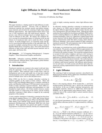
Figure 3: The convolution technique is robust for a wide range of parameters. Our method is most accurate near the source, where accuracyis most important. (left) A thick low-scattering top layer covering a highly scattering thinner lower layer. (middle) A thin low-scattering toplayer over a highly scattering thin bottom. (right) A thin highly scattering top layer over a very thick substrate. There is no transmittancesince it is optically thick.MaterialFigure 3 leftFigure 3 middleFigure 3 no-KM0.90%0.42%3.5%8.4%0.0%0.0%Table 2: Comparison of the total reflectance and transmission predicted by the multipole models to Monte Carlo for the materials inFigure 3, with and without the correction described in Section 2.3.effectively equates the impulse response of a slab to its diffuse response. Note that the multipole gives the impulse response of aslab.We can combine the profiles of two different layers by assumingthat all interactions between the two layers are due to multiple scattering. This assumption is reasonably accurate as long as diffusiontheory is applicable to the individual layers — i.e. they have a thickness of at least a few mean free paths. Based on this assumption,we can compute the profile T12 of the light transmitted through twoslabs with transmittance profiles T1 and T2 by convolving the profilesZ Z T12 (r) T1 (r0 )T2 (r00 )dx0 dy0 T1 (r) T2 (r),(18)pwhere r0 x02 y02 . This equation assumes that light transmittedthrough layer 1 onto layer 2 is transmitted through layer 2. This isnot entirely correct, since some of the light may transmit throughlayer 1, and later return to layer 1 after scattering in layer 2. Thislight can again scatter back to layer 2 and transmit out the bottomof the slab. To account for these additional scattering events at theinterface we correct Equation (18) by additional terms accountingfor each scattering event:T12 T1 T2 T1 R2 R1 T2 T1 R2 R1 R2 R1 T2 . . .(19)where we have omitted the dependence on r for brevity. This seriesof convolutions can be evaluated efficiently using Fourier theory,which changes each convolution into a product in frequency spaceT12 T1 T2 T1 R2 R1 T2 T1 R2 R1 R2 R1 T2 . . . T1 T2 (1 R2 R1 (R2 R1 )2 (R2 R1 )3 . . .), (20)where R and T are Fourier transformed diffuse reflectance andtransmittance profiles. The resulting expression is a geometric series. Assuming that R1 R2 1, we can simplify Equation 20 toT12 T1 T2.1 R2 R1(21)A similar analysis to above produces a similar formula for the reflectance of two layersR12 R1 T1 R2 T1.1 R2 R1(22)This method can be extended to more than two layers by recursive substitution of Equations (21) and (22) in for R1 or T1 , andre-evaluating the formulas. The real-space reflectance and transmittance profiles of a many-layered material is computed by computingthe inverse Fourier transform of the total frequency response.Note that these formulas are identical to Kubelka’s [1954], but applied in frequency space. They can also be considered as an application of the multipole approximation as a scattering function inoperator form [Pharr and Hanrahan 2000].Figure 3 compares the convolution of the responses of two-layeredmaterials, and a comparison to Monte Carlo photon tracing. Theconvolution of the two layers closely approximates the reflectanceand transmittance profiles near the source, and though it can diverge slightly far from the source, the intensity levels are not significant. Table 2 shows the effect of frequency space correction.Note that with correction, the total reflectance and transmittanceprofiles more closely matches the Monte Carlo simulations.2.4Rough surfacesOur derivation so far has assumed that the top surface of the material is smooth. We can account for rough surfaces by modifying theboundary condition that states how the diffused light is reflected atthe surface. This can be done by replacing the Fresnel term in Equation (5) by an appropriate BRDF. In the following, we will assumethat a microfacet model can be used to describe the roughness ofthe surface, and we model the surface reflection using a TorranceSparrow BRDF [Torrance and Sparrow 1967] o, ω i) fr (x, ω o, ω i )G(x, ω o, ω i )F(x, ω i, ω o)D(x, ω,4( ωi · n)( ωo · n)(23)
where n is the surface normal, and D, G, and F are the facet distribution, geometric term, and the Fresnel term (see [Glassner 1995]for details). In the case of a smooth surface the diffuse Fresnel term,Fdr , given in Equation (8) specifies the fraction of diffuse light reflected at the surface. In the case of a rough surface we replace thisterm by an average diffuse reflection, ρd . For the Torrance-Sparrowmodel there is no analytic approximation of the diffuse reflection,and we compute it using Monte Carlo sampling by evaluating theBRDF for random diffuse incident directions and averaging the resulting value for the reflection (this is done once for a given material).Once the diffuse reflection factor, ρd , is computed we can modifythe A term (Equation 7) used in the computation of the extrapolationdistance as follows:1 ρdA .(24)1 ρdIn addition, Equation (2) is changed by replacing both Fresnel termswith a diffuse transmission function i ; xo , ω o) Sd (xi , ω1 i )R( xi xo )ρdt (xo , ω o ),ρ (xi , ωπ dt(25)where o ) 1.0 ρdt (x, ωZ2π o, ω i )( fr (x, ωωi · n) d ωi .(26)We assume all light that is not reflected by the BRDF model istransmitted into the material. Since ρdt is a fairly smooth function, we use numerical integration and generate a small table fordifferent incoming angles. The use of ρdt is an approximation, asthe transmitted light has a directional distribution described by aBRDF for transmitted light [Stam 2001]. Since we use a diffusionmodel, however, this distribution can be ignored, and we considerall transmitted light to be diffuse.(a few mean-free paths) geometry it is possible to blend the reflection and transmission profiles, depending on the normals nl and nsat the location of the incident light and the point being shadedPd (r) 12 ( ns · nl 1)Rd (r) 21 (1 ns · nl )Td (r) .This equation computes a new profile as the weighted average of thereflected and transmitted profiles. Note that only the reflected profile is used if the normals point in the same direction, while only thetransmitted profile is used if they point in opposite directions. Onepotential improvement to this formula would be to take into accountthe relative position of the two points as well (e.g. if the normals arefacing each other). However, since the geometry between the pointbeing shaded and the point being illuminated is unknown, there isno guarantee of accuracy. For applications that require high degreesof precision for small complex geometry, it is better to use MonteCarlo photon tracing or a multi-grid diffusion solver.3.1A simpler technique that works well in practice is to assume that thetexture is given as an albedo map (e.g. diffuse reflectance) similarto textures used to shade opaque materials. This approach has beenused on translucent materials based on the dipole model [Jensen andBuhler 2002; Hery 2003]. If we further assume that only nearbytexture values influence each other then we can account for texturing using the following approach. First, we convolve the texture with the reflectance profile (andthe transmittance profile if thin geometry is being shaded).This effectively blurs the texture according to the diffusion oflight (a similar approach has been used on the irradiance valueby Borshukov et al. [2003]). Next, we normalize the texture such that the average is a whitecolor. This is done to ensure that the color of the diffusionprocess is used, rather than the texture color. If the texturecolor is important then the texture can be normalized by thereflectance and/or transmittance value predicted by the multipole method (we have not used this approach).Rendering with the Multi-Layer ModelThe multi-layered diffusion model is computed by evaluating themultipole for each layer, and using the Fourier transform techniquedescribed in the previous section to obtain the total diffuse transmittance and reflectance of the material. Because no analytical transform of the multipole equation exists, we use the discrete Fouriertransform to generate tabulated reflectance and transmittance profiles. Discretely sampling the profiles is computational efficientcompared to re-evaluating the multipole for every pixel. This isparticularly beneficial when capturing the properties of highly scattering extremely thin layers, where a large number of dipole pairsmay be required. For thicker, less scattering single slabs, the analytic multipole model can be used directly. Both the analytic multipole and the tabulated profiles can be rendered using the sametechniques as the dipole method.The multi-layer model provides both a reflectance and a transmittance profile, but the geometry to be rendered determines how theyshould be used. As with the dipole model these profiles are onlyvalid for planar slabs, and can only be used as approximations forother types of geometry. When modeling a multi-layered materialsuch as skin it is sufficient in most cases to use only the reflectanceprofile to model the diffusion of light. In the case of complex thinTexturingTexturing a multi-layered translucent material can be done in anumber of ways. If the texture contains information about the scattering properties of each layer then it is possible to approximate thespatially varying reflectance and transmittance profiles by convolving the spatially varying reflectance and/or transmittance profilesfor the individual layers (assuming that the surface is locally homogeneous). This process is costly as it has to be done for every pointon the surface or for every texture element.The final model for the appearance of a rough translucent materialconsists of the diffusion model plus the BRDF for the reflection oflight by the rough surface. As the surface roughness increases thismodel predicts that less light will be transmitted into the material,while more light is reflected directly by the surface. This results ina desaturation of the color of the translucent material as the importance of the (often white) surface reflection grows.3(27) Finally, during rendering we compute the effective diffusionof light using the reflectance and/or transmittance profile, andscale the predicted radiant emittance by the normalized texture value.4Results and DiscussionWe have implemented the multi-layered diffusion model in a MonteCarlo ray tracer that supports direct sampling of scattering profilesas described in [Jensen et al. 2001]. The images were rendered ona 2.8GHz Pentium IV, and the rendering times for the individualimages were from one to five minutes. Preprocessing time to generate the scattering profiles ranged from five seconds to under onesecond, using 1000 dipole pairs to ensure accuracy.Figure 4 compares the accuracy of the multipole method with thedipole method and Monte Carlo photon tracing. The scene containsa thin piece of parchment illuminated from behind. The parchmentis roughly 1 mm. thick, which corresponds to approximately fourmean free paths. The dipole predicts a transmittance of about 3.3%compared with 22.6% for the multipole and 21.5% for the Monte
Dipole modelMultipole modelMonte Carlo referenceFigure 4: A piece of parchment illuminated from behind. Note,how the dipole model (left) underestimates the amount of transmitted light, while the multipole model (middle) matches the referenceimage computed using Monte Carlo photon tracing (right).Front and back, frontlit.Front and back, backlit.Figure 6: A layered leaf lit from front and behind. The reflectanceof the front and back sides of the leaf differ significantly, while thetransmittance is nearly identical. Note that the color is due to multiple scattering; no textures are applied.epidermisupper dermisbloody dermisσa (mm 1)σsRGBR2.12.15.0 48.00.160.19 0.30 32.00.0851.025.0 4.5(mm 1)GBηg60.0 65.0 1.4 0.040.0 46.0 1.34 0.254.74.8 1.4 0.8d (mm).03.05 Table 3: Optical parameters used in generating the images in Figure 8. η is the index of refraction, and d is the thickness of the layer.JadeJade paintFigure 5: A buddha statuette sprayed with a thin layer of whitepaint. The first and third images are front-lit, the second and fourthback-lit.Carlo reference result. As a consequence, the parchment is too darkwhen rendered with the dipole diffusion model, while the multipolemodel more precisely predicts the correct appearance.Figure 5 shows the effect of adding a thin layer of paint onto athicker buddha statue made of jade. The paint is highly scatteringof white light, while the jade absorbs most non-green light. Addingthe paint layer causes the reflected light to become more white, andattenuates the amount of light that reaches the jade, causing thestatue to look more opaque. The transmitted light, however, remains green as it still scatters through the jade material.Figure 7 demonstrates several renderings of a marble statue withdifferent surface roughness values. As the surface roughness increases, the surface changes from having an oily appearance tolooking more dry and rough. Another important change is the desaturation of the color of the statue due to an increase in the amountof reflected light, and a reduction in the amount of lighting due tosubsurface scattering.Figure 6 displays renderings of a leaf composed of a thick absorbing layer over a thin highly scattering layer, similar to [Hemenger1977], with absorption parameters taken from [Fukshansky et al.1993]. Note that while the orientation of the leaf affects the reflectance, the transmittance is nearly the same. This bicoloration isan important visual element of many leaves. For the leaf model, weapplied both thickness and bump maps on the geometry to simulatethe appearance
model of single scattering in layered materials. Stam [2001] ex-amined the total subsurface reflectance and transmittance of a slab bounded by rough surfaces. All of these models, however, assume that light scatters at a single point on the surface, and the resulting subsurface