Transcription
142IEEE TRANSACTIONS ON ANTENNAS AND PROPAGATION, VOL. 56, NO. 1, JANUARY 2008Electric Field Integral Equations for ElectromagneticScattering Problems With Electrically Small andElectrically Large RegionsBenjamin D. Braaten, Student Member, IEEE, Robert M. Nelson, Senior Member, IEEE, andMaqsood A. Mohammed, Senior Member, IEEEAbstract—Numerically stable electric field integral equations(EFIE) are presented for electromagnetic scattering problemsthat may include both electrically small geometrically complexand electrically large regions. A reduced integrand is achieved byimplementing quasi-static assumptions in the electrically smallregions, full-wave methods in the electrically large regions, andapplying appropriate coupling relations between the regions. Useof the method provides computational efficiency as well as insightinto the conditions under which the electromagnetic fields withinelectrically small regions of the problem can be assumed to beprimarily capacitive or inductive in nature. The theoretical development of the method is highlighted in this communication andthen applied to examples of electrically small, inductively-loaded,and capacitively-loaded monopole antennas. The accuracy of theresults is verified with two independent methods.Index Terms—Hybrid solution methods, method of moments(MoM), scattering.I. INTRODUCTIONLECTROMAGNETIC waves impinging on a body inspace may induce surface currents on that body, whichproduce a scattered field. One method of determining the magnitude and phase of the scattered field is to establish and solvea set of integral equations for the unknown surface currents andcharges [1]. Once these induced currents and charges are determined, the scattered field can be evaluated. The application ofsuch concepts has been carried out for years using techniquessuch as the method of moments (MoM) [2]. Although usedfor many types of problems, it has been noted that applicationof full-wave techniques to electrically small, geometricallycomplex problems can lead to numerical instability [3].Previous authors [3]–[5] have shown that certain simplifyingassumptions are reasonable for problems with both electricallylarge and electrically small regions that may be geometricallycomplex and contain multiple types of material. For such problems, it has been shown that employing quasi-static equationsEManuscript received August 30, 2005; revised August 23, 2007.B. D. Braaten and R. M. Nelson were with the Department of Electricaland Computer Engineering, North Dakota State University, Fargo, ND 58105USA and also with Jacobs Technology, Inc., Eglin AFB, FL 32542 USA. Theyare now with the Department of Electrical and Computer Engineering, NorthDakota State University, Fargo, ND 58105 USA (e-mail: r.m.nelson@ieee.org).M. A. Mohammed is with the TEAS Group, Jacobs Technology, Inc., EglinAFB, FL 32542 USA.Digital Object Identifier 10.1109/TAP.2007.912941in the electrically small regions, full-wave methods in the remaining regions and appropriately coupling the regions provides solution improvements that include improved numericalefficiency via using a reduced quasi-static Green’s function,reduction of the number of unknowns to a single scalar(rather than up to two vector unknowns if full-wave techniquesare used throughout), and reduction of numerical difficultiesassociated with solving electrically small problems using fullwave techniques [3]–[5]. This technique has been called the hybrid quasi-static/full-wave method [4] and was previously limited to problems that exhibited axial symmetry and had electrically small regions in which magnetic induction effects couldbe ignored.In this work, the hybrid quasi-static/full-wave method developed by Olsen, Hower, and Mannikko has been re-visited.All original equations have been re-derived, Matlab-based computer code has been developed and significant new work hasbeen undertaken. The primary goal of this work is to significantly extend the applicability of the method to general casesthat exhibit both inductive and capacitive effects in the electrically small regions.As such, the method can now be used to model a host of problems that involve both electrically large conducting objects andelectrically small, geometrically complex regions. Examples ofproblems include any type of “large” metal structure (e.g., VLFantenna system, high-voltage power line, aircraft or weapon systems, cabling between electronic systems, etc.) that might alsohave “small” regions (e.g., insulators, radomes, passive circuits,etc.). In addition to providing a means of solving such problems, the work also provides insight into the conditions underwhich the electromagnetic fields within an electrically small region of the problem can be assumed to be primarily capacitiveor inductive in nature. Understanding this can have a markedinfluence on the choice of methods used to minimize undesirable effects (i.e., electromagnetic interference) [6], [7]. This insight also paves the way for future work involving lumped-element modeling (i.e., use of the method to derive equivalent circuit parameters). In the process of achieving this primary goal,all of the computational advantages previously cited have beenpreserved.II. DERIVATION OF THE EFIEConsider the geometry of the general electromagneticsproblem shown in Fig. 1. The problem consists of four distinctlinear, homogeneous, isotropic regions. Regions 1 and 2 are0018-926X/ 25.00 2008 IEEE
BRAATEN et al.: EFIES FOR ELECTROMAGNETIC SCATTERING PROBLEMS143bounding the th region of interest (note that the integral is aprinciple value integral [8], [9]). The primed vectors representthe source points and the unprimed vectors represent the fieldpoints. takes on the values of 1 and 2 in the following mannerif and are within region andif is on[3]:the smooth boundary surface of the region containing .In this work, we are interested in solving the general problemdefined by (1)–(3) for scenarios that involve both electricallylarge and electrically small regions (which may be geometrically complex and characterized by finite values of permittivityand permeability). As mentioned earlier, dividing such problems into the electrically large and electrically small regions notonly offers computational advantages but also provides the opportunity to investigate whether the electromagnetic fields inelectrically small regions are predominantly capacitive or inductive in nature. To facilitate modeling such problems, we willhenceforth assume that regions 2 and 4 are electrically small andregion 3 is electrically large.A. Quasi-Static EquationsFig. 1. General electromagnetics problem.assumed lossless, characterized by the respective values ofpermittivity and permeability. Regions 3 and 4 are assumed tobe perfect conductors. In Fig. 1 it is important to note that thedashed lines show expanded views of selected regions. Notealso that region 1 is the unbounded space surrounding the otherthree regions—which might be entirely in the full-wave region,or partly in the full-wave region and partly in the quasi-staticregion. Lastly, it should be noted that region 3 can be directlyconnected to region 1, 2 or 4. In terms of the equations thatdenotes the smooth surface between regions i andfollowj. denotes the vector measured from an arbitrary coordinatesystem defined on the general electromagnetics problem anddenotes the unit normal vector in the same coordinate systempointing into the th region. The th region has permittivityand permeability; and on the subsurfacethere exists an impressed electric field representinga source in the region. The electric field for in the th regioncan be written as [3](1)Note that (1)–(3) indicate that the electric field in the ith region can be expressed in terms of surface integrals evaluatedover all surfaces bounding that region. As such, a few approximations can be made if both the field points and source pointsare in the same quasi-static region. Assumeis the overallmaximum dimension of the quasi-static region. If the field pointis in region 1 or region 2 of the quasi-static region, and if, then. This then gives.1Thus foror 2 (3) can be written as(4)This approximation greatly reduces the kernel of the electricfield integral equations (EFIE) in the quasi-static regions andprovides a considerable gain in computational efficiency andstability over the full-wave version [3]. For this situation,can be written as(5)whereis the vectorfrom the source point to the field point. This also gives(6)whereWith these approximations (2) can be written as(2)and(7)(3), and. Equation (1) assumes thatandthere are no volume sources defined in the problem. Also, theand indifields in (1) and (2) are assumed to vary withcates that the integral is evaluated over all the smooth surfacesTo evaluate the new EFIE a general expression for the electricfield needs to be determined. Consider regions 1 and 2 in Fig. 1.1Lossless regions are assumed in this work. The efficacy of using complexmaterial constants to account for loss will be examined in the future by evaluating this approximation when k is complex.
144IEEE TRANSACTIONS ON ANTENNAS AND PROPAGATION, VOL. 56, NO. 1, JANUARY 2008Using (1), if is in the quasi-static region (i.e.,electric field in region 1 can be written asthe(8)Similarly, the electric field in region 2 can be written as(9)for not in region , a general expression forSincethe electric field in the quasi-static region can be written as [10]Fig. 2. Boundary limit for the EFIE in the quasi-static region.onshown in Fig. 2. To evaluate this boundary conditionat , the limits [10], [11](10)Employing the boundary conditionsandonandthatallows one to write (10) as [11](13)ononand notingforand 2and(14)are evaluated withfrom region 1 along the dottedfrom region 2 along the dottednormal vector andnormal vector in Fig. 2.givesSubtracting (14) from (13) and solving for[10]–[13](11)where(12)(15)Notice that the approximation in (4) is not used in (12). This isbecause the source points are in the full-wave region and not inthe same quasi-static region. Also notice that the expressionsfor (or on. The tangential components of the magneticfields in (15) are continuous across[13] and are related toand total surfacethe polarization surface current [14] onand. Thus a direct subtraction of (14) fromcurrents on(13) gives the three integrands in (15) for the tangential magnetic fields. The normal components of the electric fields in (15)and are related to the polarizationare discontinuous acrossand total surface charge onand.surface charge onThe third term on the right hand side of (15) is due to the dis[11].continuity of the normal components acrossandrepresent the magnetic inductive effects. These terms were assumed negligible in earlier work [3], [4].B. Material Interfaces Within the Quasi-Static Regionin the expression for the electric field in (11), theUsingis enforced at pointboundary conditionC. Conductor Interfaces Within the Quasi-Static RegionThe next boundary condition to be enforced ison. Using (5) and (11) the boundary condition for the electricfield is(16)
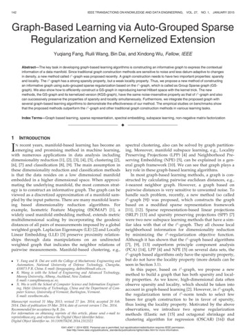
BRAATEN et al.: EFIES FOR ELECTROMAGNETIC SCATTERING PROBLEMS145where(17)andFig. 3. Enforcement of current continuity equation and conservation of charge.(18)E. Conductor Interfaces in Full-Wave RegionandoninUsing the boundary conditionFig. 1, the expression for the electric field can be written as(19)Equation (18) is the term that represents the inductive effects inthe quasi-static region which were assumed negligible for thecases considered by Olsen, Hower, and Mannikko [3], [4]. A.similar relation exists for onD. Full-Wave EquationsConsider the conductor interfaces in the full-wave region.Using the equivalence theorem the expression for the electricfield in region 1 can be written as(24)F. Current Continuity and Conservation of ChargeThe unknowns in the previous equations include surfacecharge density in the quasi-static region and surface currentdensity in both regions. These unknowns are related via theconservation of charge and current continuity equation. Consider a completely connected conductor which might lie partlyin the full-wave region and partly in the quasi-static region.The conservation of free charge for this conductor is enforcedthrough(20)(25)is the expression for the electric field from sources onandin the quasi-static region and can be writtenas(21)with(22)whereis collection of all quasi-static surfaces,isthe collection of all full-wave surfaces, and is the coordinatealong a surface. is the total free charge on the conductor andis assumed to be zero for our problems. Since current is the onlyunknown to be determined in the full-wave region, the currentcontinuity equation is used to express the charge in the full-waveregion in terms of the current. The continuity equation is(26)and(23)andare the surfacewherecurrent and total (free and polarization) surface charge densities,respectively on each surface.where and are the surface current and total surface chargedensities on each surface.Consider the axially symmetric problem in Fig. 3 to help illustrate the use of the current continuity equation and the conservation of charge. It consists of a full-wave region and a quasi-staticregion that are connected with a conductor. The quasi-static region also has an additional subregion that contains a lossless
146IEEE TRANSACTIONS ON ANTENNAS AND PROPAGATION, VOL. 56, NO. 1, JANUARY 2008material. If we assume that the current in Fig. 3 is axially symmetric and has no azimuthal component, we can write (26) as(27)iswhere is a coordinate measured along the surface andthe amplitude of the surface current flowing on the surface at .Since the only unknown in the full-wave region is current, wewill need the integral form of (27) which is expressed in termsof both current and charge(28)whereis the current at either boundary ( or ) of theis the current along the fullquasi-static region, and againwave surface at the coordinate . (28) is the integration of (27)from either boundary between the two electrical regions to theandcoordinate . Thus, multiplying both sides of (25) byusing (28) we eliminate the need to solve for the charge in thefull-wave region.For example, by making the previous substitution and assuming that the current at the end of the full-wave conductors isand) and region 1 iszero (i.e.,free space, we can write(29)whereandare the transitional currents betweenthe full-wave region and the quasi-static region. (29) enforcesthe continuity of current between the two electrical regions. Itshould be noted that the current at the boundaries between thequasi-static regions and full-wave regions is not assumed to bezero. This allows the coupling between different electrical regions to be computed. Special care should be taken while computing these boundary currents. Another place where specialcare must be exercised is at junctions between perfect conductors and general lossless materials, such as node in Fig. 3. We, only polarization (ornote that only free charge exists on, and both exist on. For such inbound) charge exists onstances (25) and (28) are applied to account for free charge, anda modified form is applied a second time to account for polarization (or bound) charge.If the problem has only full-wave regions then the enforcement of (28) is not needed. The use of (24) without the last termcan be used to solve for the desired unknowns. On the otherhand if the problem of interest has only quasi-static regions thenthe enforcement of (25) and (28) is required to solve for theunknowns.Now (15), (16), (24), (25), and (28) can be solved for thecurrents and charges in all regions.III. COMPUTATIONAL EXAMPLES AND CONSIDERATIONSHaving laid the theoretical foundation for the new workwe turn to computational aspects. We begin by looking atspecific examples which highlight the primary focus of thisFig. 4. Inductively loaded monopole.work—namely to determine the solution of scattering problemsthat include both electrically large and electrically small regions(which may exhibit both inductive and capacitive effects). Wealso examine various computational considerations includinginsights regarding how the number of equations, unknowns,and computational speed compare to full-wave methods, aswell as when it may be appropriate to model the effect of theelectromagnetic fields within electrically small regions usingtwo-terminal circuit elements. Such insights lay the foundationfor future work that may focus directly on using two-terminalcircuit elements to model such situations.A. Computational ExamplesThe first problem selected to test the new EFIE was the inductively loaded monopole shown in Fig. 4. Part of the quasi-staticregion in Fig. 4 is a ferrite bead wrapping around a wire. Suchbeads are often used to introduce inductance [6], [7]. In thisproblem, the “ferrite bead” region is characterized byand permeabilitywithmm andmm. We note thatalso provides correct results, butwas used so that the 4th term on the right side of(15) is non-zero.As implied by the reference to a ferrite bead, this problemwas selected because it exhibits significant inductive effects. Itis not always clear if the electromagnetic fields in quasi-staticregions are primarily inductive or capacitive. Arguments to helpdetermine this are presented in [3] and will be discussed shortly.The MoM was used to solve the new EFIE. In particular, thepoint matching technique [19] was chosen. Matlab was used tocarry out the MoM implementation. The Matlab code containssubroutines that generate the source and match points, carry outnecessary numerical integration, and solve the resulting matrix equation. A Matlab-based graphical user interface (GUI)was written to help manage all the subroutines. The nameQUICNEC [11] has been given to this Matlab GUI. QUICNEC
BRAATEN et al.: EFIES FOR ELECTROMAGNETIC SCATTERING PROBLEMS147Fig. 5. Input resistance for inductively loaded monopole.Fig. 6. Input reactance for inductively loaded monopole.stands for quasi-static inductive capacitive numerical electromagnetics code. The GUI allows the user to easily input anarray of axially symmetric problems. (More information on thecapabilities and limitations of QUICNEC can be found in [11].)QUICNEC was used to determine the input impedance of theinductively loaded monopole shown in Fig. 4. The number ofunknowns was increased until the input impedance convergedin this case). It should be noted thatis larger(than what might typically be expected because both the surfacecharge density (in the quasi-static region) and surface currentdensity (in both full-wave and quasi-static regions) are beingsolved for simultaneously.The results obtained from the new EFIE are compared tothe results provided by Mininec Classic [15] and Ansoft [16].Mininec Classic was used because a lumped element can becalculated to approximate the inductance of the quasi-static region. For the geometry shown in Fig. 4 an equivalent lumpedwas used. (This expressioninductor ofcan be derived by determining the energy stored in the magneticfield within the bead, assuming a magnetic field intensity in the.) For the problem at hand, a lumpedbead ofinductance of L 15.5 nH was defined in Mininec Classic at anode that corresponded to the center of the quasi-static regionin Fig. 4. Results from QUICNEC were also compared to thoseobtained using Ansoft. Ansoft was chosen for two reasons. First,it provides results using the Finite Element Method [17] whichis based on completely different principles than presented here.Secondly, work done by Kennedy, Long, and Williams [18] suggest that solutions to problems similar to this one can be calculated using Ansoft. It should be noted here that the surfaces defined in Ansoft were not smooth. Every surface was defined tobe a tetrahedron with 14 sides.Results for the input impedance of the monopole antennawere obtained using all three methods (QUICNEC, Mininec andAnsoft) for the frequency range of 0.3–2.0 GHz. This frequencyrange was selected to ensure that the quasi-static assumptionswere still valid. The calculated input resistance and reactanceare shown in Figs. 5 and 6, respectively. Excellent correlationis noted between the results obtained from the new EFIE (i.e.,QUICNEC), Mininec Classic, and Ansoft.The input impedance of a monopole without a load is alsopresented in Figs. 5 and 6. Results obtained from the originalhybrid method [3]–[5] and those of an unloaded monopole areincluded to show the significance of the inductive effects. Theseresults suggest that using a two-terminal inductive element torepresent the effect of the electromagnetic fields in this regionis justified. As such, the capacitive effects in this region can beneglected.The results shown in Figs. 5 and 6 clearly illustrate the efficacy of the work presented here for problems involving inductive effects. Several other types of problems have been also beenexamined. The capacitively loaded monopole shown in [3] wassimulated using the EFIE described here and in [11]. The results compare very well with measurement results and resultsobtained from the original hybrid quasi-static/full-wave [3].Initial results have also been obtained for lossy materials byusing complex values of and to account for loss. Althoughthe outcome of these simulations look promising [21], furtherwork needs to be undertaken to provide a rigorous proof of theapplicability of using the new EFIE for such cases.B. Computational ConsiderationsThe primary focus of this work was to extend the applicability of the original hybrid quasi-static/full-wave method to include both inductive and capacitive effects in electrically smallregions. This method provides the user with the opportunityof not only solving complex problems, but also being able toinvestigate if the electromagnetic fields in the quasi-static region are predominantly capacitive or inductive in nature. To examine that question, we note that the relative magnitudes ofthe first and third terms in (7) can be shown to beandrespectively. Ifthencapacitive effects are dominant in the quasi-static regions [3].inductive effects are dominant. IfIfthen both terms need to be considered.imIf capacitive effects are dominant,plies that. As Olsen points out [3], [4] sincewithin the electrically small region, this inequalityis “large”, which implies thatwill hold wheneverhas significant spacial variation within the region. This will be
148IEEE TRANSACTIONS ON ANTENNAS AND PROPAGATION, VOL. 56, NO. 1, JANUARY 2008true when the current changes rapidly. An example given in [3],[4] is that of a parallel plate capacitor where “the current variesrapidly near the capacitor plates to sustain a build up of charge”[3], [4].To gain further insight into the capacitive problem, note that. Therefore, capacitive effects are(26) implies. Sincein the elecdominant whentrically small region, if “ ” means a factor of less than or equal. Noting thatto 0.1 (a typical assumption),becomes.Therefore, capacitive effects are dominant when(30)Although (30) provides a description of the relative magnitudesof the surface charge and current for capacitively dominantproblems, it does not yield a useful prediction mechanismsince these magnitudes are not known a priori. A similar resultwill occur for problems where inductive effects are dominant.Although it may not be possible to determine if capacitive orinductive effects are dominant a priori, the results presentedhere can be used to provide meaningful insight for particularproblems. One way to check this is to run QUICNEC and thenrun a modified form of QUICNEC which neglects the inductivein (16) and then compare the results.effects in (15) andIf negligible changes in the results occur, the effects were predominantly capacitive for that problem. If significant changesoccur in the results one can conclude that significant inductiveeffects occurred. For example, capacitive effects were verifiedin the case of the capacitively loaded monopole by observingno change in the input impedance when the two versions ofQUICNEC were run. For the example of the inductively loadedmonopole, very significant changes were observed in the resultsobtained from the two versions of QUICNEC. This indicatesthat significant inductive effects are present. Although onecannot definitely say that capacitive effects are negligible, thesignificant change in results indicates this may be the case. Forthe particular results shown in Fig. 5 dominant inductive effectsare verified by the excellent agreement between the QUICNECresults (i.e., the new EFIE) and those obtained with the othermethods. Further work is in progress which will allow the userto determine definitively whether inductive or capacitive effectsare dominant for a given problem.Although the main focus of this work was not to reduce thenumber of unknowns or decrease computation time, improvement in such aspects were welcome benefits. To examine suchissues, consider the equations that need to be solved if one usestraditional full-wave techniques to enforce the boundary conditions on a dielectric-dielectric interface. It can be shown [1] thatthe resulting equations are(31)and(32),andis given in (3). Ifwhereis obtained using the current continuity equation one needsto solve 5 equations with 5 unknowns (i.e., two components of, along with ). In contrast, (15) is the equationboth andenforced on the dielectric-dielectric interfaces in the quasi-staticregions, which results in one equation and three unknowns (i.e.,, along with ). For a general quasitwo components ofstatic problem, the other two equations are obtained by applying(29) to each component of . Thus application of this methodto general dielectric-dielectric interfaces reduces the problemfrom solving 5 scalar equations to 3 scalar equations for eachsurface. Note that the number of unknowns for both methods arereduced if azimuthal currents are neglected (such as in thin-wireproblems).In addition to reducing the number of equations and unknowns, it is important to note that the integrands within thenew EFIE are less complex than those in the full-wave methoddescribed by (31) and (32). Each of the full-wave integrands inbut in (15) the correspondingvolve terms with either orandterms, whichquasi-static equation involves theresult in decreased computation time. Therefore, the methodpresented here results in fewer unknowns for the quasi-staticregions, and reduced computational burden for a given numberof unknowns. We point out that the equations used to enforcethe boundary condition on the conductor-dielectric interfacewill yield the same number of unknowns for both the full-waveand quasi-static versions of the EFIE. For instance, (16) willyield 3 unknowns (surface charge and two components ofsurface current) and two equations. The third equation is (26).Although the number of unknowns for the dielectric-conductorinterface is the same for both EFIE, the quasi-static integrandswill have less computational burden than the correspondingfull-wave integrands. To illustrate that fact, we compare computation times when a full-wave code and QUICNEC are bothused to evaluate the problem shown in Fig. 7. It consists ofa perfectly conducting quasi-static cylinder withand. The problem was evaluated using Harrington’sfull-wave EFIE ([2, Ch. 4]) and our quasi-static EFIE withthe current continuity equation. We used the point matchingtechnique with pulse basis functions and solved for the current and charge. The surface charge calculated using the twomethods correspond very well with the exception of the sourcelocation (which is a common characteristic of the delta source[22]). Now we want to compare the cpu time between the twomethods. Table I shows the average cpu time for each N. Inboth routines we solve for both the current and charge. Anaverage of 56.66 percent less cpu time was realized with thequasi-static EFIE over the full-wave EFIE.
BRAATEN et al.: EFIES FOR ELECTROMAGNETIC SCATTERING PROBLEMS149ACKNOWLEDGMENTThe authors would like to thank Dr. R. G. Olsen (WashingtonState University) for providing a copy of the Fortran code basedon the work in [3] and [4]. They would also like to thank theCenter for Nanoscale Science and Engineering (CNSE), NorthDakota State University, for providing access to Ansoft, whichwas used to verify results given in this work.REFERENCESFig. 7. Quasi-static region.TABLE ICPU COMPUTATION TIMEIV. CONCLUSIONAn integral equation technique has been successfully developed to compute the fields from scattering problems that mayhave both quasi-static and full-wave regions. The quasi-staticregions are considered electrically small and can consist ofgeometries and material characteristics with permittivities andpermeabilities of unity or greater. A MoM implementation hasbeen carried out in Matlab. Results of the input impedanceof an inductively loaded monopole are presented and compared with those obtained using Mininec Classic and Ansoft.Excellent correlation is obtained—verifying that the new integral equations provide accurate, detailed results for quasi-staticregions with significant inductive and capacitive effects. Useof the method also provides insight into the conditions underwhich the electromagnetic fields within electrically small regions can be assumed to be primarily capacitive or inductive.Computational considerations are addressed, which includes acomparison of CPU times required for the new EFIE and atraditional full-wave EFIE to determine the surface charge andcurrent for an electrically small wire. Computational efficiencyis noted.[1] R. A. Mittra, Ed., Computer Techniques for Electromagnetics. Washington, DC: Hemisphere Publishing, 1987, pp. 159–182.[2] R. F. Harrington, Field Computation by Moment Methods. Malabar,FL: Krieger Publishing, 1982.[3] R. G. Olsen, G. L. Hower, and P. D. Mannikko, “A hybrid method forcombining quasi-static and full-wave techniques for electroma
142 IEEE TRANSACTIONS ON ANTENNAS AND PROPAGATION, VOL. 56, NO. 1, JANUARY 2008 Electric Field Integral Equations for Electromagnetic Scattering Problems With Electrically Small and Electrically Large Regions Benjamin D. Braaten, Student Member, IEEE, Robert M. Nelson, Senior Member, IEEE, and