WIXLIB

PrologueThe discipline of statistics deals with the collection and analysis of data. Advancesin computing technology, particularly in relation to changes in science and business,have increased the need for more statistical scientists to examine the huge amountof data being collected. We know that data are not equivalent to information. Oncedata (hopefully of high quality) are collected, there is a strong need for statisticiansto make sense of them. That is, data must be analyzed in order to provide information upon which decisions can be made. In light of this great demand, opportunitiesfor the discipline of statistics have never been greater, and there is a special need formore bright young persons to go into statistical science.If we think of fields in which data play a major part, the list is almost endless:accounting, actuarial science, atmospheric science, biological science, economics,educational measurement, environmental science, epidemiology, finance, genetics,manufacturing, marketing, medicine, pharmaceutical industries, psychology, sociology, sports, and on and on. Because statistics is useful in all of these areas, it reallyshould be taught as an applied science. Nevertheless, to go very far in such an appliedscience, it is necessary to understand the importance of creating models for each situation under study. Now, no model is ever exactly right, but some are extremelyuseful as an approximation to the real situation. Most appropriate models in statistics require a certain mathematical background in probability. Accordingly, whilealluding to applications in the examples and the exercises, this textbook is reallyabout the mathematics needed for the appreciation of probabilistic models necessaryfor statistical inferences.In a sense, statistical techniques are really the heart of the scientific method.Observations are made that suggest conjectures. These conjectures are tested, anddata are collected and analyzed, providing information about the truth of theconjectures. Sometimes the conjectures are supported by the data, but often theconjectures need to be modified and more data must be collected to test the modifications, and so on. Clearly, in this iterative process, statistics plays a major rolewith its emphasis on the proper design and analysis of experiments and the resultinginferences upon which decisions can be made. Through statistics, information is provided that is relevant to taking certain actions, including improving manufacturedproducts, providing better services, marketing new products or services, forecastingenergy needs, classifying diseases better, and so on.Statisticians recognize that there are often small errors in their inferences, andthey attempt to quantify the probabilities of those mistakes and make them as smallas possible. That these uncertainties even exist is due to the fact that there is variationin the data. Even though experiments are repeated under seemingly the same conditions, the results vary from trial to trial. We try to improve the quality of the data bymaking them as reliable as possible, but the data simply do not fall on given patterns.In light of this uncertainty, the statistician tries to determine the pattern in the bestpossible way, always explaining the error structures of the statistical estimates.This is an important lesson to be learned: Variation is almost everywhere. It isthe statistician’s job to understand variation. Often, as in manufacturing, the desire isto reduce variation because the products will be more consistent. In other words, carvii

viii Prologuedoors will fit better in the manufacturing of automobiles if the variation is decreasedby making each door closer to its target values.Many statisticians in industry have stressed the need for “statistical thinking”in everyday operations. This need is based upon three points (two of which havebeen mentioned in the preceding paragraph): (1) Variation exists in all processes;(2) understanding and reducing undesirable variation is a key to success; and (3)all work occurs in a system of interconnected processes. W. Edwards Deming, anesteemed statistician and quality improvement “guru,” stressed these three points,particularly the third one. He would carefully note that you could not maximizethe total operation by maximizing the individual components unless they are independent of each other. However, in most instances, they are highly dependent, andpersons in different departments must work together in creating the best productsand services. If not, what one unit does to better itself could very well hurt others.He often cited an orchestra as an illustration of the need for the members to worktogether to create an outcome that is consistent and desirable.Any student of statistics should understand the nature of variability and thenecessity for creating probabilistic models of that variability. We cannot avoid making inferences and decisions in the face of this uncertainty; however, these inferencesand decisions are greatly influenced by the probabilistic models selected. Somepersons are better model builders than others and accordingly will make better inferences and decisions. The assumptions needed for each statistical model are carefullyexamined; it is hoped that thereby the reader will become a better model builder.Finally, we must mention how modern statistical analyses have become dependent upon the computer. Statisticians and computer scientists really should worktogether in areas of exploratory data analysis and “data mining.” Statistical softwaredevelopment is critical today, for the best of it is needed in complicated data analyses. In light of this growing relationship between these two fields, it is good advicefor bright students to take substantial offerings in statistics and in computer science.Students majoring in statistics, computer science, or a joint program are in greatdemand in the workplace and in graduate programs. Clearly, they can earn advanceddegrees in statistics or computer science or both. But, more important, they arehighly desirable candidates for graduate work in other areas: actuarial science, industrial engineering, finance, marketing, accounting, management science, psychology,economics, law, sociology, medicine, health sciences, etc. So many fields have been“mathematized” that their programs are begging for majors in statistics or computerscience. Often, such students become “stars” in these other areas. We truly hope thatwe can interest students enough that they want to study more statistics. If they do,they will find that the opportunities for very successful careers are numerous.

Chap terChapter1Probability1.11.21.3Properties of ProbabilityMethods of EnumerationConditional Probability1.41.5Independent EventsBayes’ Theorem1.1 PROPERTIES OF PROBABILITYIt is usually difficult to explain to the general public what statisticians do. Many thinkof us as “math nerds” who seem to enjoy dealing with numbers. And there is sometruth to that concept. But if we consider the bigger picture, many recognize thatstatisticians can be extremely helpful in many investigations.Consider the following:1. There is some problem or situation that needs to be considered; so statisticiansare often asked to work with investigators or research scientists.2. Suppose that some measure (or measures) is needed to help us understandthe situation better. The measurement problem is often extremely difficult, andcreating good measures is a valuable skill. As an illustration, in higher education, how do we measure good teaching? This is a question to which we havenot found a satisfactory answer, although several measures, such as studentevaluations, have been used in the past.3. After the measuring instrument has been developed, we must collect datathrough observation, possibly the results of a survey or an experiment.4. Using these data, statisticians summarize the results, often with descriptivestatistics and graphical methods.5. These summaries are then used to analyze the situation. Here it is possible thatstatisticians make what are called statistical inferences.6. Finally, a report is presented, along with some recommendations that are basedupon the data and the analysis of them. Frequently such a recommendationmight be to perform the survey or experiment again, possibly changing some ofthe questions or factors involved. This is how statistics is used in what is referredto as the scientific method, because often the analysis of the data suggests otherexperiments. Accordingly, the scientist must consider different possibilities inhis or her search for an answer and thus performs similar experiments over andover again.1

2 Chapter 1 ProbabilityThe discipline of statistics deals with the collection and analysis of data. Whenmeasurements are taken, even seemingly under the same conditions, the results usually vary. Despite this variability, a statistician tries to find a pattern; yet due to the“noise,” not all of the data fit into the pattern. In the face of the variability, thestatistician must still determine the best way to describe the pattern. Accordingly,statisticians know that mistakes will be made in data analysis, and they try to minimize those errors as much as possible and then give bounds on the possible errors.By considering these bounds, decision makers can decide how much confidence theywant to place in the data and in their analysis of them. If the bounds are wide, perhaps more data should be collected. If, however, the bounds are narrow, the personinvolved in the study might want to make a decision and proceed accordingly.Variability is a fact of life, and proper statistical methods can help us understanddata collected under inherent variability. Because of this variability, many decisionshave to be made that involve uncertainties. In medical research, interest may center on the effectiveness of a new vaccine for mumps; an agronomist must decidewhether an increase in yield can be attributed to a new strain of wheat; a meteorologist is interested in predicting the probability of rain; the state legislature mustdecide whether decreasing speed limits will result in fewer accidents; the admissionsofficer of a college must predict the college performance of an incoming freshman;a biologist is interested in estimating the clutch size for a particular type of bird;an economist desires to estimate the unemployment rate; an environmentalist testswhether new controls have resulted in a reduction in pollution.In reviewing the preceding (relatively short) list of possible areas of applicationsof statistics, the reader should recognize that good statistics is closely associated withcareful thinking in many investigations. As an illustration, students should appreciate how statistics is used in the endless cycle of the scientific method. We observenature and ask questions, we run experiments and collect data that shed light onthese questions, we analyze the data and compare the results of the analysis withwhat we previously thought, we raise new questions, and on and on. Or if you like,statistics is clearly part of the important “plan–do–study–act” cycle: Questions areraised and investigations planned and carried out. The resulting data are studied andanalyzed and then acted upon, often raising new questions.There are many aspects of statistics. Some people get interested in the subjectby collecting data and trying to make sense out of their observations. In some casesthe answers are obvious and little training in statistical methods is necessary. But ifa person goes very far in many investigations, he or she soon realizes that there is aneed for some theory to help describe the error structure associated with the variousestimates of the patterns. That is, at some point appropriate probability and mathematical models are required to make sense out of complicated data sets. Statisticsand the probabilistic foundation on which statistical methods are based can providethe models to help people do this. So in this book, we are more concerned withthe mathematical, rather than the applied, aspects of statistics. Still, we give enoughreal examples so that the reader can get a good sense of a number of importantapplications of statistical methods.In the study of statistics, we consider experiments for which the outcome cannot be predicted with certainty. Such experiments are called random experiments.Although the specific outcome of a random experiment cannot be predicted withcertainty before the experiment is performed, the collection of all possible outcomesis known and can be described and perhaps listed. The collection of all possible outcomes is denoted by S and is called the outcome space. Given an outcome spaceS, let A be a part of the collection of outcomes in S; that is, A S. Then A iscalled an event. When the random experiment is performed and the outcome of theexperiment is in A, we say that event A has occurred.

Section 1.1 Properties of Probability 3Since, in studying probability, the words set and event are interchangeable, thereader might want to review algebra of sets. Here we remind the reader of someterminology: denotes the null or empty set; A B means A is a subset of B; A B is the union of A and B; A B is the intersection of A and B; A is the complement of A (i.e., all elements in S that are not in A).Some of these sets are depicted by the shaded regions in Figure 1.1-1, in which S isthe interior of the rectangles. Such figures are called Venn diagrams.Special terminology associated with events that is often used by statisticiansincludes the following:1. A1 , A2 , . . . , Ak are mutually exclusive events means that Ai Aj , i j; thatis, A1 , A2 , . . . , Ak are disjoint sets;2. A1 , A2 , . . . , Ak are exhaustive events means that A1 A2 · · · Ak S.So if A1 , A2 , . . . , Ak are mutually exclusive and exhaustive events, we know thatAi Aj , i j, and A1 A2 · · · Ak S.Set operations satisfy several properties. For example, if A, B, and C are subsetsof S, we have the following:Commutative LawsA B B AA B B ASASAB(b) A B(a) A SSAABBC(c) A BFigure 1.1-1 Algebra of sets(d) A B C

4 Chapter 1 ProbabilityAssociative Laws(A B) C A (B C)(A B) C A (B C)Distributive LawsA (B C) (A B) (A C)A (B C) (A B) (A C)De Morgan’s Laws(A B) A B (A B) A B A Venn diagram will be used to justify the first of De Morgan’s laws. InFigure 1.1-2(a), A B is represented by horizontal lines, and thus (A B) is theregion represented by vertical lines. In Figure 1.1-2(b), A is indicated with horizontal lines, and B is indicated with vertical lines. An element belongs to A B if it belongs to both A and B . Thus the crosshatched region represents A B .Clearly, this crosshatched region is the same as that shaded with vertical lines inFigure 1.1-2(a).We are interested in defining what is meant by the probability of event A,denoted by P(A) and often called the chance of A occurring. To help us understandwhat is meant by the probability of A, consider repeating the experiment a numberof times—say, n times. Count the number of times that event A actually occurredthroughout these n performances; this number is called the frequency of event Aand is denoted by N (A). The ratio N (A)/n is called the relative frequency of eventA in these n repetitions of the experiment. A relative frequency is usually very unstable for small values of n, but it tends to stabilize as n increases. This suggests that weassociate with event A a number—say, p—that is equal to the number about whichthe relative frequency tends to stabilize. This number p can then be taken as the number that the relative frequency of event A will be near in future performances of theexperiment. Thus, although we cannot predict the outcome of a random experimentwith certainty, if we know p, for a large value of n, we can predict fairly accuratelythe relative frequency associated with event A. The number p assigned to event A isBA(a)BA(b)Figure 1.1-2 Venn diagrams illustratingDe Morgan’s laws

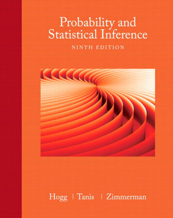
Section 1.1 Properties of Probability 5called the probability of event A and is denoted by P(A). That is, P(A) representsthe proportion of outcomes of a random experiment that terminate in the event Aas the number of trials of that experiment increases without bound.The next example will help to illustrate some of the ideas just presented.Example1.1-1A fair six-sided die is rolled six times. If the face numbered k is the outcome on rollk for k 1, 2, . . . , 6, we say that a match has occurred. The experiment is called asuccess if at least one match occurs during the six trials. Otherwise, the experimentis called a failure. The sample space is S {success, failure}. Let A {success}. Wewould like to assign a value to P(A). Accordingly, this experiment was simulated500 times on a computer. Figure 1.1-3 depicts the results of this simulation, and thefollowing table summarizes a few of the results:nN (A)N (A)/n50370.740100690.6902501720.6885003300.660The probability of event A is not intuitively obvious, but it will be shown in Example1.4-6 that P(A) 1 (1 1/6)6 0.665. This assignment is certainly supported bythe simulation (although not proved by it).Example 1.1-1 shows that at times intuition cannot be used to assign probabilities, although simulation can perhaps help to assign a probability empirically. Thenext example illustrates where intuition can help in assigning a probability to 00Figure 1.1-3 Fraction of experiments having at least onematch

6 Chapter 1 ProbabilityExample1.1-2A disk 2 inches in diameter is thrown at random on a tiled floor, where each tileis a square with sides 4 inches in length. Let C be the event that the disk will landentirely on one tile. In order to assign a value to P(C), consider the center of the disk.In what region must the center lie to ensure that the disk lies entirely on one tile?If you draw a picture, it should be clear that the center must lie within a squarehaving sides of length 2 and with its center coincident with the center of a tile.Since the area of this square is 4 and the area of a tile is 16, it makes sense to letP(C) 4/16.Sometimes the nature of an experiment is such that the probability of A canbe assigned easily. For example, when a state lottery randomly selects a three-digitinteger, we would expect each of the 1000 possible three-digit numbers to have thesame chance of being selected, namely, 1/1000. If we let A {233, 323, 332}, thenit makes sense to let P(A) 3/1000. Or if we let B {234, 243, 324, 342, 423, 432},then we would let P(B) 6/1000, the probability of the event B. Probabilities ofevents associated with many random experiments are perhaps not quite as

While this strong probability coverage of the course is important for all students, it has been particularly helpful to actuarial students who are studying for Exam P in the Society of Actuaries’ series (or Exam 1 of the Casualty Actuarial Society). The greatest change to this edition is in the s