WIXLIB

0.2 Why do we need a mathematical theory?3To illustrate the pitfalls of an intuitive approach to probability, let us consider a seemingly plausible definition. You probably think of the probabilitythat an event E happens as the fraction of outcomes in which E occurs (thisis not entirely unreasonable). We could posit this as a tentative definitionProbability of E Number of outcomes where E occurs.Number of all possible outcomesThis sort of intuitive definition may look at first sight like it matches yourexperience. However, it is totally meaningless: we can easily use it to come toentirely different conclusions.Example 0.2.1. Suppose that we flip two coins. What is the probability thatwe obtain one heads (H) and one tails (T )? Solution 1: The possible outcomes are HH, HT, T H, T T . The outcomeswhere we have one heads and one tails are HT, T H. Hence,Probability of one heads and one tails 12 .42Solution 2: The possible outcomes are two heads, one heads and one tails,two tails. Only one of these outcomes has one heads and one tails. Hence,Probability of one heads and one tails 1.3Now, you may come up with various objections to one or the other of thesesolutions. But the fact of the matter is that both of these solutions are perfectly reasonable interpretations of the “intuitive” attempt at a definition ofprobability given above. (While our modern understanding of probability corresponds to Solution 1, the eminent mathematician and physicist d’Alembertforcefully argued for Solution 2 in the 1750s in his famous encyclopedia). Wetherefore immediately see that an intuitive approach to probability is notadequate. In order to reason reliably about random phenomena, it is essential to develop a rigorous mathematical foundation that leaves no room forambiguous interpretation. This is the goal of probability theory:Probability theory is the mathematical study of random phenomena.It took many centuries to develop such a theory. The first steps in this directionhave their origin in a popular pastime of the 17th century: gambling (I suppose it is still popular). A French writer, Chevalier de Méré, wanted to knowhow to bet in the following game. A pair of dice is thrown 24 times; shouldone bet on the occurence of at least one double six? An intuitive computationled him to believe that betting on this outcome is favorable, but repeated “experiments” led him to the opposite conclusion. De Méré decided to consult hisfriend, the famous mathematician Blaise Pascal, who started correspondingabout this problem with another famous mathematician, Pierre de Fermat.

40 IntroductionThis correspondence marked the first serious attempt at understanding probabilities mathematically, and led to important works by Christiaan Huygens,Jacob Bernoulli, Abraham de Moivre, and Pierre-Simon de Laplace in thenext two centuries. It was only in 1933, however, that a truly satisfactorymathematical foundation to probability theory was developed by the eminentRussian mathematician Andrey Kolmogorov. With this solid foundation inplace, the door was finally open to the systematic development of probabilitytheory and its applications. It is Kolmogorov’s theory that is used universallytoday, and this will also be the starting point for our course.0.3 This courseIn the following chapter, we are going to develop the basic mathematicalprinciples of probability. This solid mathematical foundation will allow us tosystematically build ever more complex random models, and to analyze thebehavior of such models, without running any risk of the type of ambiguousconclusions that we saw in the example above. With precision comes necessarily a bit of abstraction, but this is nothing to worry about: the basicprinciples of probability are little more than “common sense” properly formulated in mathematical language. In the end, the success of Kolmogorov’stheory is due to the fact that it genuinely captures our real-world observationsabout randomness.Once we are comfortable with the basic framework of probability theory,we will start developing increasingly sophisticated models of random phenomena. We will pay particular attention to models of random processes wherethe randomness develops over time. The notion of time is intimately relatedwith randomness: one can argue that the future is random, but the past isnot. Indeed, we already know what happened in the past, and thus it is perfectly predictable; on the other hand, we typically cannot predict what willhappen in the future, and thus the future is random. While this idea mightseem somewhat philosophical now, it will lead us to notions such as randomwalks, branching processes, Poisson processes, Brownian motion, and Markovchains, which form the basis for many complex models that are used in numerous applications. At the end of the course, you might want to look back atthe humble point at which we started. I hope you will find yourself convincedthat a mathematical theory of probability is worth the effort.· · ·This course is aimed at a broad audience and is not a theorem-proof stylecourse.2 That does not mean, however, that this course does not require rigorous thinking. The goal of this course is to teach you how to reason preciselyabout randomness and, most importantly of all, how to think probabilistically.2Students seeking a mathematician’s approach to probability should take ORF 526.

1Basic Principles of ProbabilityThe goal of this chapter is to introduce the basic ingredients of a mathematicaltheory of probability that will form the basis for all further developments. Aswas emphasized in the introduction, these ingredients are little more than“common sense” expressed in mathematical form. You will quickly becomecomfortable with this basic machinery as we start using it in the sequel.1.1 Sample spaceA random experiment is an experiment whose outcome cannot be predictedbefore the experiment is performed. We do, however, know in advance whatoutcomes are possible in the experiment. For example, if you flip a coin, youknow it will come up either heads or tails; you just do not know which ofthese outcomes will actually occur in a given experiment.The first ingredient of any probability model is the specification of allpossible outcomes of a random experiment.Definition 1.1.1. The sample space Ω is the set of all possible outcomesof a random experiment.Example 1.1.2 (Two dice). Consider the random experiment of throwing onered die and one blue die. We denote by (i, j) the outcome that the red diecomes up i and the blue die comes up j. Hence, we define the sample spaceΩ {(i, j) : 1 i, j 6}.In this experiment, there are only 62 36 possible outcomes.

61 Basic Principles of ProbabilityExample 1.1.3 (Waiting for the bus). Consider the random experiment of waiting for a bus that will arrive at a random time in the future. In this case, theoutcome of the experiment can be any real number t 0 (t 0 means thebus comes immediately, t 1.5 means the bus comes after 1.5 hours, etc.) Wecan therefore define the sample spaceΩ [0, [.In this experiment, there are infinitely many possible outcomes.Example 1.1.4 (Flight of the bumblebee). A bee is buzzing around, and wetrack its flight trajectory for 5 seconds. What possible outcomes are there insuch a random experiment? A flight path of the bee might look somethinglike this:PositionTime012345(Of course, the true position of the bee in three dimensions is a point in R3 ; wehave plotted one coordinate for illustration). As bees have not yet discoveredthe secret of teleportation, their flight path cannot have any jumps (it mustbe continuous), but otherwise they could in principle follow any continuouspath. So, the sample space for this experiment can be chosen asΩ {all continuous paths ω : [0, 5] R3 }.This is a huge sample space. But this is not a problem: Ω faithfully describesall possible outcomes of this random experiment.1.2 EventsOnce we have defined all possible outcomes of a random experiment, we shoulddiscuss what types of questions we can ask about such outcomes. This leads usto the notion of events. Informally, an event is a statement for which we candetermine whether it is true or false after the experiment has been performed.Before we give a formal definition, let us consider some simple examples.Example 1.2.1 (Two dice). In Example 1.1.2, consider the following event:“The sum of the numbers on the dice is 7.”

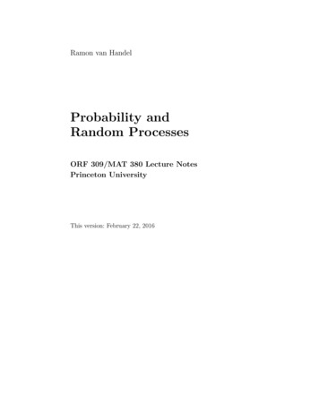
1.2 Events7Note that this event occurs in a given experiment if and only if the outcome ofthe experiment happens to lie in the following subset of all possible outcomes:{(1, 6), (2, 5), (3, 4), (4, 3), (5, 2), (6, 1)} Ω.We cannot predict in advance whether this event will occur, but we can determine whether it has occured once the outcome of the experiment is known.Example 1.2.2 (Bus). In Example 1.1.3, consider the following event:“The bus comes within the first hour.”Note that this event occurs in a given experiment if and only if the outcome ofthe experiment happens to lie in the following subset of all possible outcomes:[0, 1] Ω.Example 1.2.3 (Bumblebee). In Example 1.1.4, suppose there is an object (say,a wall or a chair) that takes up some volume A R3 of space. We want toknow whether or not the bee will hit this object in the first second of its flight.For example, we can consider the following event:“The bumblebee stays outside the set A in the first second.”Note that this event occurs in a given experiment if and only if the outcome ofthe experiment happens to lie in the following subset of all possible outcomes:{continuous paths ω : [0, 5] R3 : ω(t) 6 A for all t [0, 1]} Ω.As the above examples show, every event can be naturally identified withthe subset of all possible outcomes of the random experiment for which theevent is true. Indeed, take a moment to convince yourself that the verbaldescription of events (such as “the bus comes within an hour”) is completelyequivalent to the mathematical description as a subset of the sample space(such as [0, 1]). This observation allows us to give a formal definition.Definition 1.2.4. An event is a subset A of the sample space Ω.The formal definition allows us to translate our common sense reasoningabout events into mathematical language.Example 1.2.5 (Combining events). Consider two events A, B. The intersection A B is the event that A and B occur simultaneously.It might be helpful to draw a picture:

81 Basic Principles of ProbabilityΩABA BThe set A Ω consists of all outcomes for which the event A occurs,while B Ω consists of all outcomes for which the event B occurs.Thus A B is the set of all outcomes for which both A and B occur. The union A B is the event that A or B occurs:ΩABA B(When we say A or B, we mean that either A or B or both occur.) The complement Ac : Ω\A is the event that A does not occur:ΩAAcAlong the same lines, any common sense combination of events can betranslated into mathematical language. For example, the event “A occurs orat most one of B, C and D occur” can be written as (why?)A ((B C)c (B D)c (C D)c ).After a bit of practice, you will get used to expressing common sense statements in terms of sets. Conversely, when you see such a statement in termsof sets, you should always keep the common sense meaning of the statementin the back of your mind: for example, when you see A B, you should automatically read that as “the events A and B occur,” rather than the muchless helpful “the intersection of sets A and B.”

1.3 Probability measure91.3 Probability measureWe have now specified the sample space Ω of all possible outcomes, and theevents A Ω about which we can reason. Given these ingredients, how doesa random experiment work? Each time we run a random experiment, thegoddess of chance Tyche (Τύχη) picks one outcome ω Ω from the set ofall possible outcomes. Once this outcome is revealed to us, we can check forany event A Ω whether or not that event occurred in this realization of theexperiment by checking whether or not ω A.Unfortunately, we have no way of predicting which outcome Tyche will pickbefore conducting the experiment. We therefore also do not know in advancewhether or not some event A will occur. To model a random experiment, wewill specify for each event A our “degree of confidence” about whether thisevent will occur. This degree of confidence is specified by assigning a number0 P(A) 1, called a probability, to every event A. If P(A) 1, then weare certain that the event A will occur: in this case A will happen every timewe perform the experiment. If P(A) 0, we are certain the event A will notoccur: in this case A never happens in any experiment. If P(A) 0.7, say,then the event will occur in some realizations of the experiment and not inothers: before we run the experiment, we are 70% confident that the eventwill happen. What this means in practice is discussed further below.In order for probabilities to make sense, we cannot assign arbitrary numbers between zero and one to every event: these numbers must obey somerules that encode our common sense about how random experiments work.These rules form the basis on which all of probability theory is built.Definition 1.3.1. A probability measure is an assignment of a numberP(A) to every event A such that the following rules are satisfied.a. 0 P(A) 1 (probability is a “degree of confidence”).b. P(Ω) 1 (we are certain that something will happen).c. If A, B are events with A B , thenP(A B) P(A) P(B)(the probabilities of mutually exclusive events add up).More generally, if events E1 , E2 , . . . satisfy Ei Ej for all i 6 j,! [XPEi P(Ei ).i 1i 1

101 Basic Principles of ProbabilityRemark 1.3.2 (Probabilities, frequencies, and common sense). You probablyhave an intuitive idea about what probability means. If we flip a coin manytimes, then the coin will come up heads roughly half the time. Thus we say thatthe probability that the coin will come up heads is one half. More generally,our common sense intuition about probabilities is in terms of frequency: if werepeated a random experiment many times, the probability of an event is thefraction of these experiments in which the event occurs.The problem with this idea is that it is not clear how to use it to definea precise mathematical theory: we saw in the introduction that a heuristicdefinition in terms of fractions can lead to ambiguous conclusions. This iswhy we do not define probabilities as frequencies. Instead, we make an unambiguous mathematical definition of probability as a number P(A) assigned toevery event A. We encode common sense into mathematics by insisting thatthese numbers must satisfy some rules that are precisely the properties thatfrequencies should have. What are these rules?a. The fraction of experiments in which an event occurs must obviously, bydefinition, be a number between 0 and 1.b. As Ω is the set of all possible outcomes, the fraction of experiments wherethe outcome lies in Ω is obviously 1 by definition.c. Let A and B be two events such that A B :ΩABThis means that the events A and B can never occur in the same experiment: these events are mutually exclusive. Now suppose we repeated theexperiment many times. As A and B cannot occur simultaneously in thesame experiment, the number of experiments in which A or B occurs isprecisely the sum of the number of experiments where A occurs and whereB occurs. Thus the fraction of experiments in which A B occurs is the sumof the fraction of experiments in which A occurs and in which B occurs. Asimilar conclusion holds for mutually exclusive events E1 , E2 , . . .These three properties of frequencies are precisely the rules that we requireprobability measures to satisfy in Definition 1.3.1. Once again, we see thatthe basic principles of probability theory are little more than common senseexpressed in mathematical language.Some of you might be concerned at this point that we have traded mathematics for reality: by making a precise mathematical definition, we had to giveup our intuitive interpretation of probabilities as frequencies. It turns out that

1.3 Probability measure11this is not a problem even at the philosophical level. Even though we havenot defined probabilities in terms of frequencies, we will later be able to proveusing our theory that when we repeat an experiment many times, an event ofprobability p will occur in a fraction p of the experiments! This important result, called the law of large numbers, is an extremely convincing sign that havemade the “right” definition of probabilities: our unambiguous mathematicaltheory manages to reproduce our common sense notion of probability, whileavoiding the pitfalls of a heuristic definition (as in the introduction). We willprove the law of large numbers later in this course. In the meantime, you canrest assured that our mathematical definition of probability faithfully reproduces our everyday experience with randomness.Our definition of a probability measure requires that probabilities satisfysome common sense properties. However, there are many other common senseproperties that are not listed in Definition 1.3.1. It turns out that the threerules of Definition 1.3.1 are sufficient: we can derive many other natural properties as a consequence. Here are two simple examples.Example 1.3.3. Let A be an event. Clearly A and its complement Ac are mutually exclusive, that is, A Ac (an event cannot occur and not occur atthe same time!) On the other hand, we have A Ac Ω by definition (in anyexperiment, either A occurs or A does not occur; there are no other options!)Hence, by properties b and c in the definition of probability measure, we have1 P(Ω) P(A Ac ) P(A) P(Ac ),which implies the common sense ruleP(Ac ) 1 P(A).You can verify, for example, that this rule corresponds to your intuitive interpretation of probabilities as frequencies. As a special case, suppose thatP(A) 1, that is, we are certain that the event A will happen. Then theabove rule shows that P(Ac ) 0, that is, we are certain that A will not nothappen. That had better be true if our theory is to make any sense!Example 1.3.4. Le

2 0 Introduction Finance and economics: stock and bond prices are inherently unpre- llworkinthe .